Hotel Booking Project

Data Visualizer

Data Analyst

Microsoft Excel

Python

Python Analysis Report: Hotel Booking

Introduction

In this report, we use Python to examine the Hotel Bookings dataset. The file includes hotel registration information such as the type of hotel, the country where the appointment is made, the arrival date, the number of visitors, and so on. Our primary goal is to examine the dataset and discover intriguing details about the bookings.

The dataset was imported into Python, and we performed exploratory data analysis (EDA) and data cleaning to understand the data better and prepare it for analysis. After that, we conducted various data analysis tasks and created visualizations to gain insights into the dataset.

This analysis has been divided into the following steps:

Importing Required Libraries

The first stage was to install the necessary libraries for data processing and visualization. To disregard any cautions, we imported pandas as pd, matplotlib.pyplot as plt, seaborn as sns, and the warnings library.

import pandas as pd

import matplotlib.pyplot as plt

import seaborn as sns

import warnings

warnings.filterwarnings('ignore')

Reading the Dataset

Next, we read the hotel bookings dataset using the pandas read_csv() function and stored it in the 'df' dataframe variable. We then used the tail(), shape(), and info() functions to get a glimpse of the data.

df = pd.read_csv('hotel_bookings 2.csv')

Exploratory Data Analysis and Data Cleaning

/ Data Cleaning

In this stage, we cleaned the data to guarantee that it was ready for analysis. To deal with the date and time objects, we used the pd.to_datetime() method to transform the reservation_status_date column to datetime format. The describe() method was then used to get the descriptive statistics of the object type columns, and a for loop was used to display the distinct numbers of each column to find any anomalies or incorrect data. We deleted the 'company' and 'agent" categories based on the information received from these methods because they had a large number of incomplete values. We also used the dropna() method to remove any rows with missing data.

Data Exploration and Visualization

1. Exploratory Data Analysis

After cleaning the data, we proceed to examine it by analyzing various categories. To get the unique numbers and total of each categorical field, we use describe (include = "object"). Then, to detect any anomalies, we display the unique numbers of each column.

2. Cancellation Analysis

Using value_counts (normalize = True) on the 'is_canceled' column, we calculate the proportion of canceled bookings. The reservation state tally is then visualized using a bar graph.

This shows that canceled reservations are less than non-canceled ones.

cancelled_percs = df['is_canceled'].value_counts(normalize = True)

print(cancelled_percs)

plt.figure(figsize = (5,4))

plt.title('Reservation status count')

plt.bar(['Not canceled','Canceled'],df['is_canceled'].value_counts(), edgecolor = 'k', width = 0.7)



plt.show()

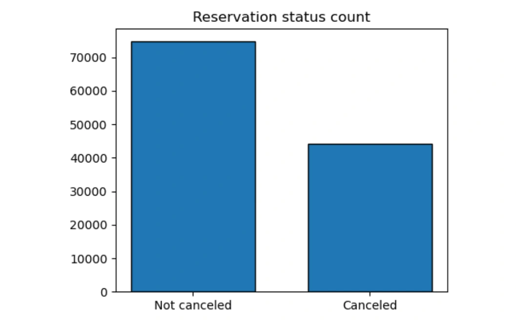
Cancelation Analysis using a bar graph

3. Hotel-wise Cancellation Analysis

Using the Seaborn library, we conduct a hotel-wise cancellation analysis by showing a countplot of the 'hotel' column. The data is then categorized by hotel type, and the cancellation rate for each hotel category is calculated. We then use a line graph to assess the average daily rate for each hotel category.

City Hotel has booked more reservations than the Resort Hotel

The City Hotel got more reservations canceled than the Resort Hotel

plt.figure(figsize = (8,4))

axl= sns.countplot(x='hotel', hue = 'is_canceled', data = df, palette = 'Blues')

legend_labels,_ = axl.get_legend_handles_labels()

#axl.legend(bbox_to_anchor(1,1))

plt.title('Reservation status in different hotels', size = 20)

plt.xlabel('hotel')

plt.ylabel('Number of reservations')

plt.show()

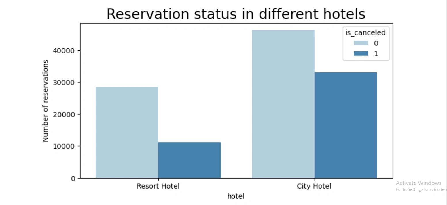
Reservation Status in City and Resort hotels

4. Cancellation Analysis by Hotel Type

We calculated the normalized value counts of the 'is_canceled' column for 'Resort Hotel' and 'City Hotel' to understand the cancellation rates for each:

resort_hotel = resort_hotel.groupby('reservation_status_date')[['adr']].mean()

city_hotel = city_hotel.groupby('reservation_status_date')[['adr']].mean()

5. Average Daily Rate (ADR) Analysis

We analyzed the Average Daily Rate (ADR) for both City and Resort Hotels over time and created a plot to visualize the trend:

plt.figure(figsize = (20,8))

plt.title('Average Daily Rate in City and Resort Hotel', fontsize = 30)

plt.plot(resort_hotel.index, resort_hotel['adr'], label = 'Resort Hotel')

plt.plot(city_hotel.index, city_hotel['adr'], label = 'City Hotel')

plt.legend(fontsize = 20)

plt.show()

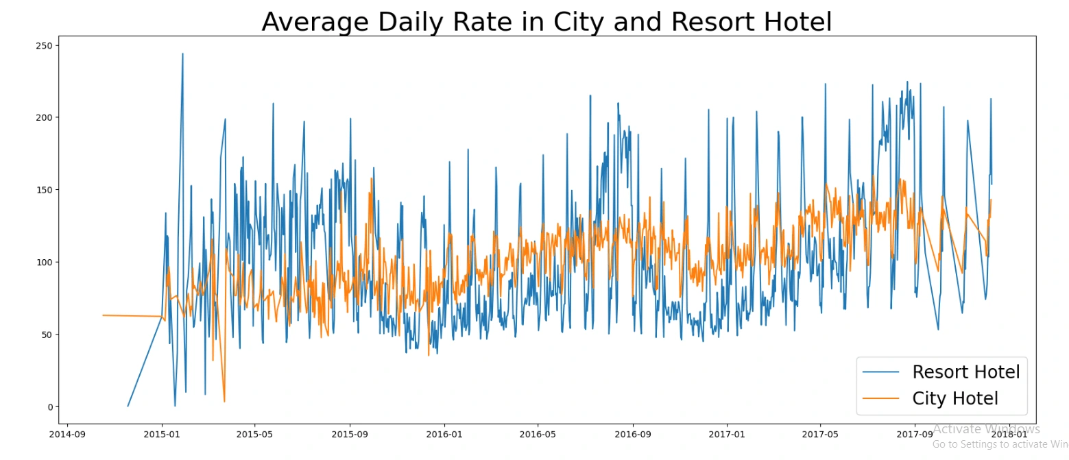
Daily rates in City and Resort hotels

6. Monthly Analysis

We examine the reservation state month by month by grouping the data and producing a countplot. We then use a bar graph to plot the average daily cost per month for canceled bookings.

df['month'] = df['reservation_status_date'].dt.month

plt.figure(figsize = (16,8))

axl = sns.countplot(x = 'month', hue = 'is_canceled', data = df)

legend_labels,_ = axl.get_legend_handles_labels()

#axl.legend(bbox_to_anchor(1,1))

plt.title('Reservation status per month', size = 20)

plt.xlabel('month')

plt.ylabel('number of reservations')

plt.legend(['not canceled', 'canceled'])

plt.show()

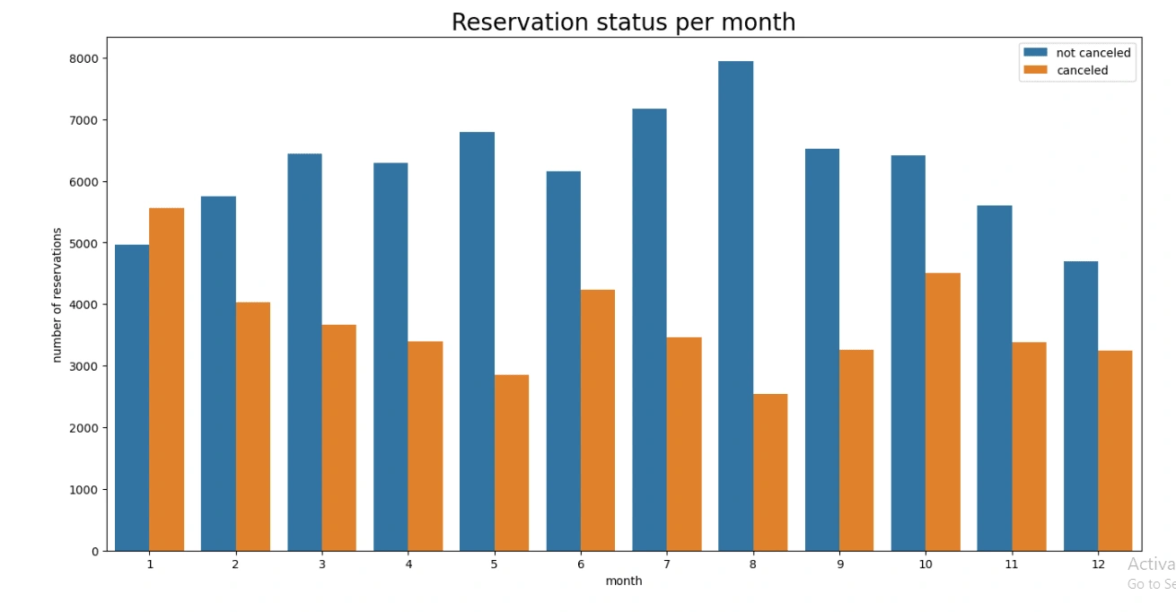
Reservation status per month

7. ADR Analysis for Canceled Reservations

We analyzed the ADR for canceled reservations and created a bar plot to visualize it:

plt.figure(figsize = (15,8))

plt.title('ADR per month', fontsize = 30)

sns.barplot('month', 'adr', data = df[df['is_canceled'] == 1].groupby('month')[['adr']].sum().reset_index())

plt.show()

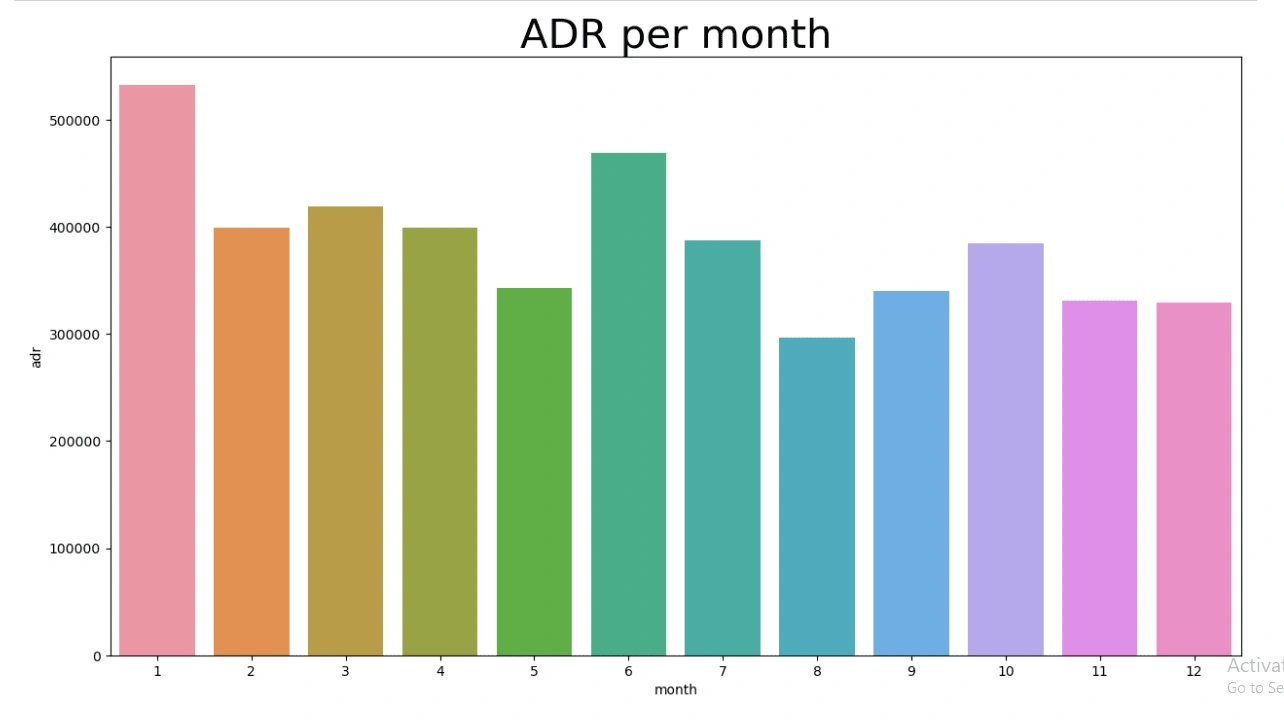
ADR per month analysis

8. Top 10 Canceled Reservations by Country

We identified the top 10 countries with the most canceled reservations and created a pie chart to visualize them.

Portugal has the largest number of Canceled Reservations with 70.07%

Great Britain comes second with 6.25%

Spain lies in 3rd with 5.54%

France has 4.93%

3.93% in Italy

3.10 in Germany

2.12% in Ireland

2.11 in Brazil

1.28% in USA

1.21% in Belgium

cancelled_data = df[df['is_canceled'] == 1]

top_10_countries = cancelled_data['country'].value_counts()[:10]

plt.figure(figsize = (8,8))

plt.title('Top 10 countries with reservation canceled')

plt.pie(top_10_countries, autopct = '%.2f',labels = top_10_countries.index)

plt.show()

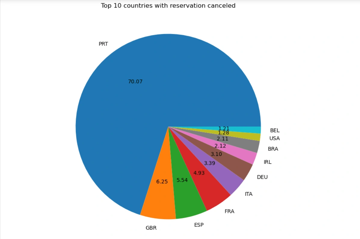
Country-wise cancellation rate

9. Market Segment Analysis

We analyzed the market segment distribution for reservations and calculated the relative frequency of each market segment:

df['market_segment'].value_counts()
df['market_segment'].value_counts(normalize=True)

cancelled_data['market_segment'].value_counts(normalize=True)

10. ADR Analysis for Canceled and Not Canceled Reservations

To further analyze the dataset, we delved into the Average Daily Rate (ADR) for both canceled and not canceled reservations.

For canceled reservations, we calculated the ADR by grouping the data by the 'reservation_status_date' column and determining the mean ADR for each date. After this, we reset the index to obtain a clean DataFrame:

cancelled_df_adr = cancelled_data.groupby('reservation_status_date')[['adr']].mean()

cancelled_df_adr.reset_index(inplace = True)

cancelled_df_adr.sort_values('reservation_status_date')

Similarly, we performed the same analysis for not canceled reservations. We filtered the dataset to select only the rows where 'is_canceled' is equal to 0 and calculated the mean ADR for each date. This operation provided insights into the ADR trends for reservations that were not canceled:


not_cancelled_data = df[df['is_canceled'] == 0]

not_cancelled_df_adr = not_cancelled_data.groupby('reservation_status_date')[['adr']].mean()

not_cancelled_df_adr.reset_index(inplace = True)

not_cancelled_df_adr.sort_values('reservation_status_date')

To visualize the ADR trends for both canceled and not canceled reservations, we created a line plot. The 'reservation_status_date' was plotted on the x-axis, while the ADR was represented on the y-axis. This visualization allowed for a clear comparison of the ADR between these two reservation categories:


plt.figure(figsize = (20,6))

plt.title('Average daily rate', fontsize = 30)

plt.plot(not_cancelled_df_adr['reservation_status_date'],not_cancelled_df_adr['adr'], label = 'not_cancelled')

plt.plot(cancelled_df_adr['reservation_status_date'],cancelled_df_adr['adr'], label = 'cancelled')

plt.legend()

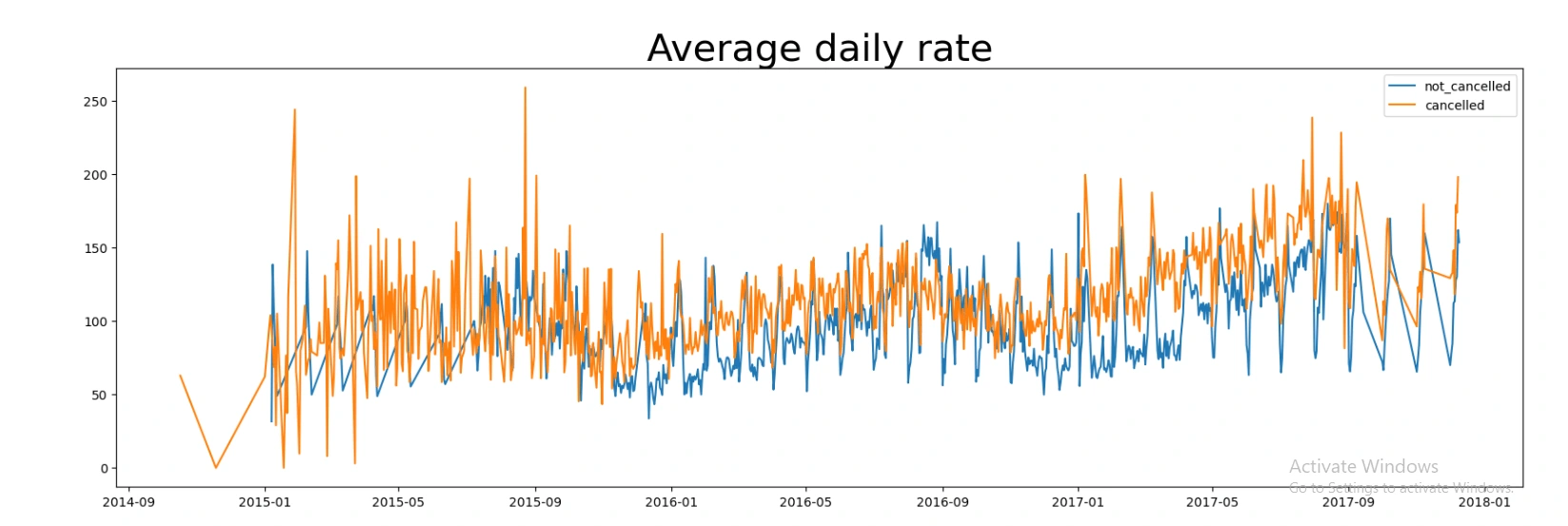
Average daily rate

In addition, we filtered the ADR data to focus on a specific time period. Both the 'cancelled_df_adr' and 'not_cancelled_df_adr' DataFrames were refined to include only rows with dates falling within the range of greater than '2016' and less than '2017-09':

cancelled_df_adr = cancelled_df_adr[(cancelled_df_adr['reservation_status_date' ] > '2016') & (cancelled_df_adr['reservation_status_date' ] < '2017-09')]

not_cancelled_df_adr = not_cancelled_df_adr[(not_cancelled_df_adr['reservation_status_date' ] > '2016') & (not_cancelled_df_adr['reservation_status_date' ] < '2017-09')]

Consequently, a line plot was created to visualize the ADR trends for this specific period, showcasing the ADR for both canceled and not canceled reservations. This provided a focused view of ADR dynamics during that time frame:

plt.figure(figsize = (20,6))

plt.title('Average daily rate', fontsize = 30)

plt.plot(not_cancelled_df_adr['reservation_status_date'],not_cancelled_df_adr['adr'], label = 'not_cancelled')

plt.plot(cancelled_df_adr['reservation_status_date'],cancelled_df_adr['adr'], label = 'cancelled')

plt.legend(fontsize = 20)

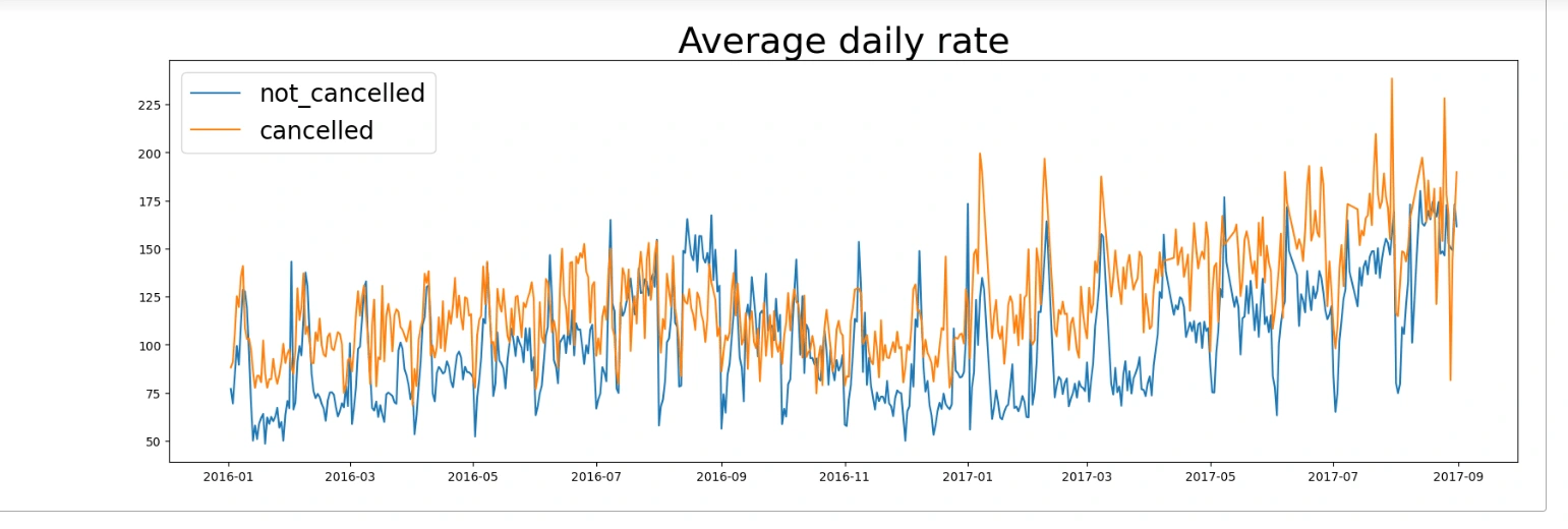
Avg daily rate from 2016-1017

These analyses and visualizations offer valuable insights into market segment distribution and ADR trends, enabling a deeper understanding of the dataset.

Conclusion

Finally, we used data analysis and visualization to obtain insight into consumer reservation trends. We discovered that the bulk of bookings were not canceled and that the cancellation rate in city hotels was greater than that in resort hotels. We also discovered that the majority of canceled reservations originated from the top ten nations. Portugal has the largest number of canceled reservations with 71.07%. We also found that the ADR for canceled reservations was cheaper than the ADR for reservations that were not canceled. Finally, we discovered that the market group with the most bookings was the Internet travel agent and that the majority of reservations were made during the summer months.