DanielOX/Data-Engineering-Workflow-DUCKDB
Danial Shabbir
Understanding NYC Taxi Trip Data
The New York City Taxi and Limousine Commission (TLC) collect extensive data concerning taxi trips within the city. This data provides a rich resource for analysis and modeling, aiding in various business and urban planning decisions. In this article, we delve into leveraging Jupyter Notebook to dissect and organize this data into meaningful Dimension and Fact tables for analytics purposes.
Dataset Download Link: https://www.nyc.gov/site/tlc/about/tlc-trip-record-data.page
Note: For the purpose of this article we will be using dataset from year 2023 (Yellow Taxi)
Introduction to the Data
The provided dataset contains detailed records of taxi trips from the year 2023 trips. It captures pivotal information such as pick-up and drop-off dates/times, trip distances, fare details, passenger counts, and more. It's important to note that this data was collected and supplied to the TLC by technology providers under authorized programs. Therefore, while being valuable, the accuracy and completeness of the dataset might not be guaranteed.
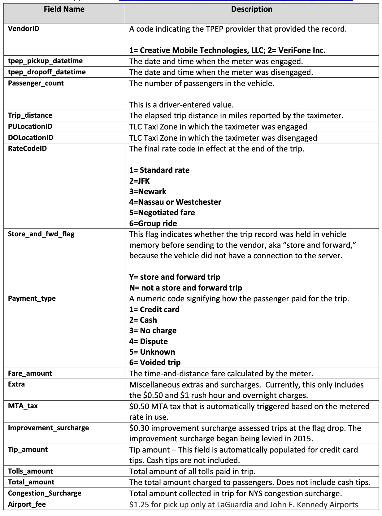
Data Dictionary or Data Catalog
Below image contains all the data points we will getting and their descriptions from the dataset.
Process Flow of the Pipeline
Loading and Data Preprocessing
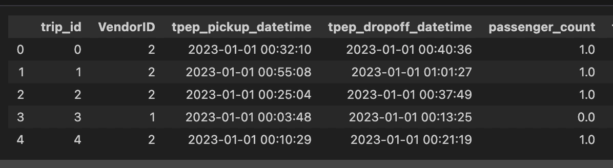
The analysis starts with loading the data into a Pandas DataFrame within the Jupyter Notebook environment. This initial step involves crucial data preprocessing tasks such as:
Checking data types and ensuring appropriate formats for date-time columns.
Removing duplicate entries to maintain data integrity.
Generating a unique Trip ID for each trip record for identification purposes. (also known as surrogate key)
Constructing Dimension Tables
Once, the data is fully cleaned. We creates dimension tables for different entities
datetime_dim: This table captures datetime-related attributes such as pickup and drop-off hours, days, months, years, and weekdays.
passenger_count_dim: Contains passenger count information.
trip_distance_dim: Holds details about trip distances.
rate_code_dim: Provides insights into different rate codes and their corresponding names.
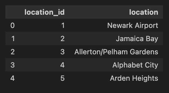
location_dim: A look-up table for location which maps locationID for pickup/dropff into location_name
pickup_location_dim: Stores data about pickup locations.
dropoff_location_dim: Holds data regarding drop-off locations.
payment_type_dim: Contains information about various payment types.
Building the Fact Table
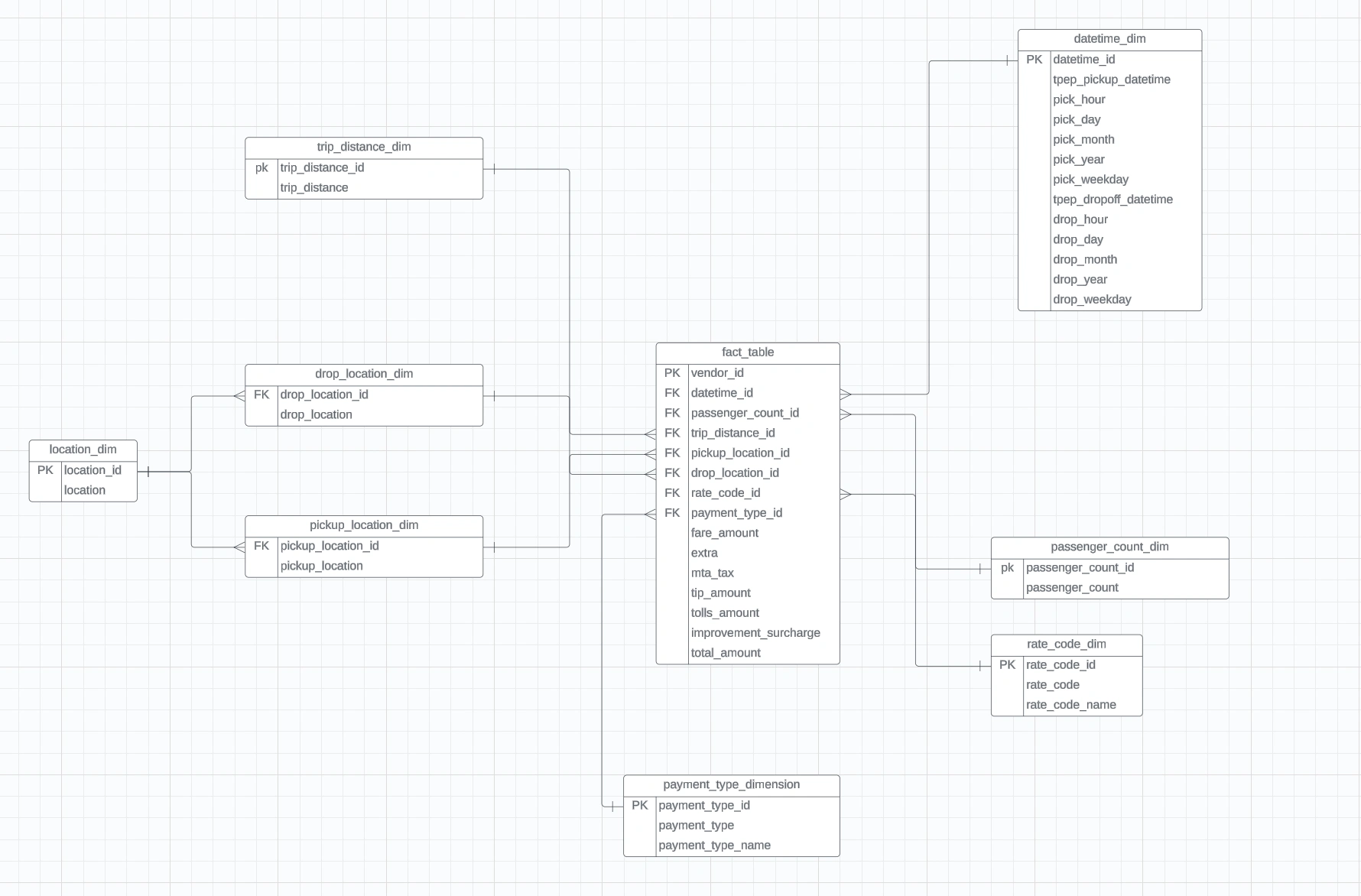
The Fact table, the heart of a dimensional model, is constructed by merging various Dimension tables. It encapsulates essential information such as trip details, fare amounts, payment details, dropoff_location_dim, pickup_location_dim, passenger details and more.
Diagram of Data Model
Some Complex Analytics using Our Data Model
We will write some analytical queries using duckdb to query data from our data model. This will present and help us identify different usecases.

Some details about parquet file format
CSV files store data in rows with values separated by delimiters, while JSON uses key-value pairs for structured data. Parquet, however, arranges data by columns, allowing more efficient storage and retrieval of column-specific information. It employs advanced compression techniques and encoding methods, like Run-Length and Dictionary Encoding, resulting in smaller file sizes and faster query performance. This optimized structure makes Parquet well-suited for analytical workloads, big data processing, and data warehousing, as it significantly reduces storage needs and enhances processing speeds compared to CSV and JSON formats.
personal note: I will always prefer working with parquet format for my analytical projects, even if the source file csv/json, i will always try to convert it into parquet format.
Preprocessing Steps & Surrogate Key
We will perform a basic preprocessing step
drop duplicates
add a surrogate key
Each record in dataset represents a trip. we can apply complex hashing (md5, sha256) of concatenating multiple columns to represent a unique record for each trip or we can just assign the monotically increasing id. Both can work, i will be applying monotonically increasing id. Pandas provide this out of the box when we load in the dataframe. it is called
index.just for the reference, if some of the folks wants to take hashing route. one can apply the logic as below. please note it's gonna be a little slow
Data Modelling
Now preprocessing of the data is completed. The next step would be to create data model.
Some definations of
data model and dimnensions in a layman term Data Model
A data model is like a blueprint or a plan that defines how data is organized, structured, and related within a database or system.
Why do we need it?
It helps in understanding the different types of data, their relationships, and how they can be accessed or retrieved.
Analogy
Imagine you're building a house. Before construction begins, you have architectural plans that detail where rooms will be located, how they connect, and what materials will be used. Similarly, a data model outlines how data will be stored, what types of data are needed, and how different pieces of data relate to each other.
Dimension
A dimension in a model refers to a way of organizing or categorizing data to help understand and analyze information more effectively. It's like grouping or labeling data based on specific attributes or characteristics.
Why do we need it?
Dimensions provide context and structure to data, making it easier to study and gain insights. They help in organizing information in a meaningful way, allowing users to ask questions and perform analyses that can lead to better decision-making.
Analogy
In a sales model, time can be a dimension. You might break down time into years, months, and days to analyze sales performance over different time periods. Similarly, in a customer model, age or location can be dimensions to categorize customers based on their age groups or geographic regions.
Creating datetime_dim dimension table
datetime_dim dimension tableNow lets build the datetime dimension as depicted in the picture. As you can see, i have broken down the time to minute, hour, day, weekday, month, year for each pickup and dropoff. This is helpful for analysing the information. An analyst is now able to gain visibility upto minute level analytics of trips. This is also called
Granularity of data.Some notes about Granularity
Granularity in simple terms means
The level of detail at which the attributes and characteristics (columns) of data are defined so the more we dive deeper the granularity of data becomes (individual level info) and the more we aggregate data the granularity becomes higher (department level info). High Granularity can be related to as seeing a whole picture (bigger view) and low level granularity means seeing individual elements of the whole picture. e.g seeing an individual salary would be lower granular and seeing the department's average salary would be high granular level of detail.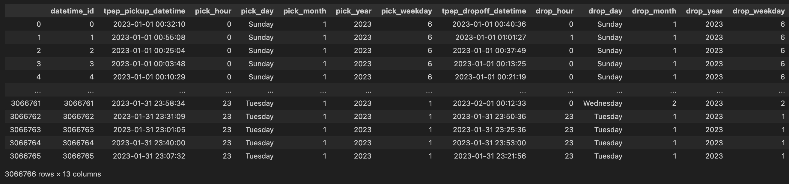
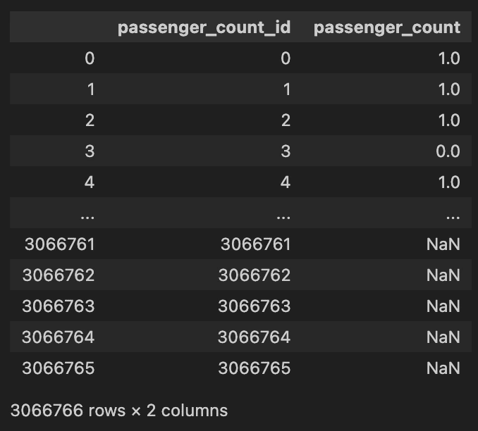
Creating passenger_count_dim dimension table
passenger_count_dim dimension table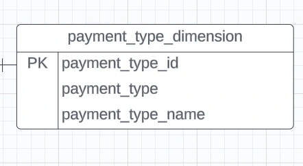
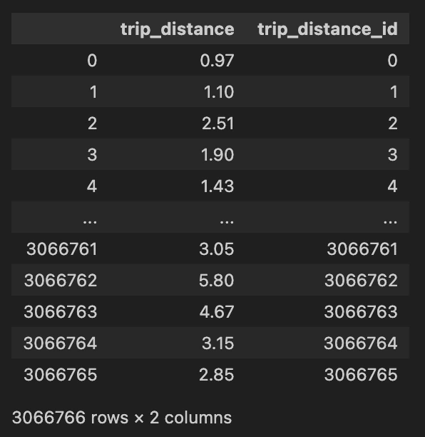
Creating trip_distance_dim dimension table
trip_distance_dim dimension table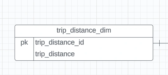
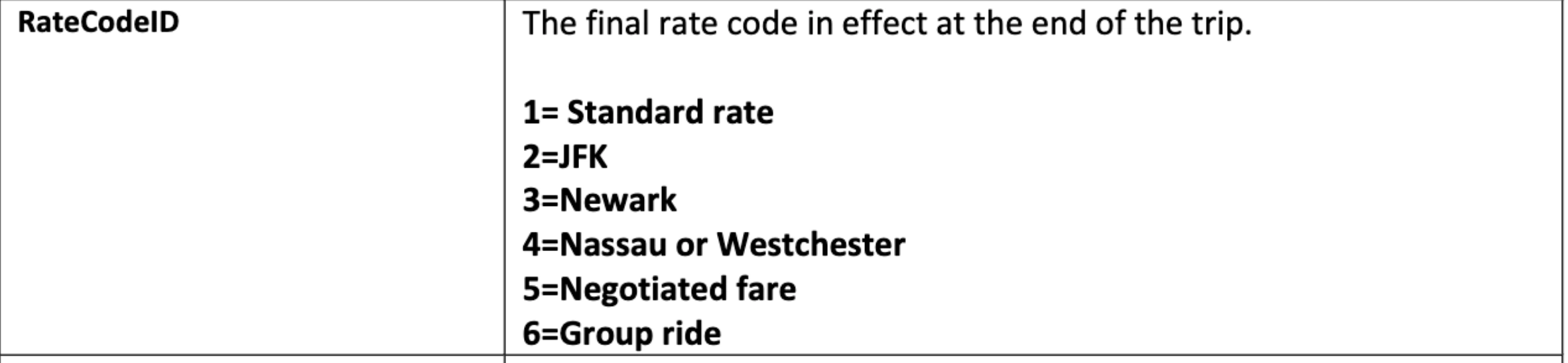
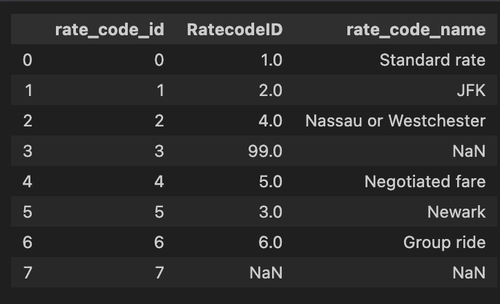
Creating rate_code_dim dimension table
rate_code_dim dimension table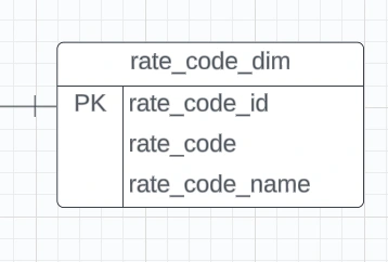
if we look in the data dictionary the information about rate code id are provided e.g 1 = 'Standard rate' etc. We can add this meta info in our dimension table to make it more helpful for our analysts.
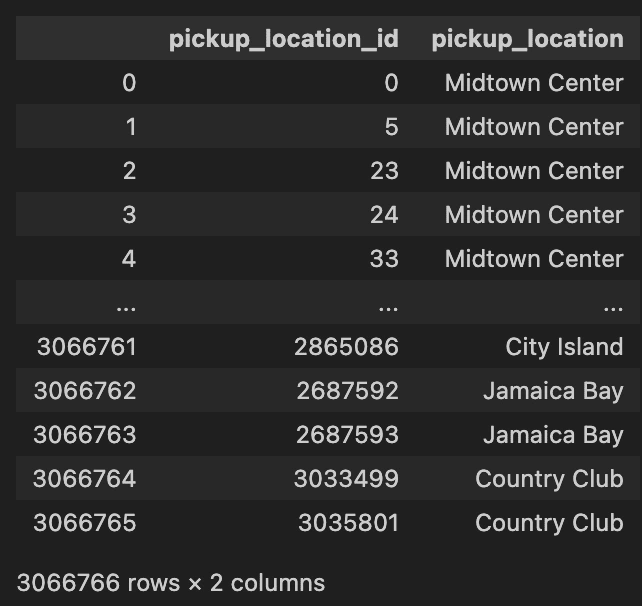
Creating pickup_location_dim dimension table
pickup_location_dim dimension tableWe have
PULocationID and DOLocationID column which doesn't mean anything to us unless we have a location name. Therefore, we will be using a lookup table which has mappings for each of location_id and their zone/location. If we refer to the above diagram, the lookup table which i am referring to is as follows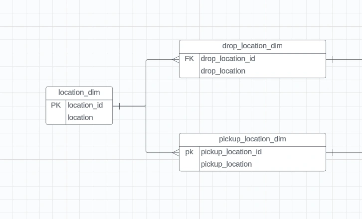
Location Dim
Creating dropoff_location_dim dimension table
dropoff_location_dim dimension table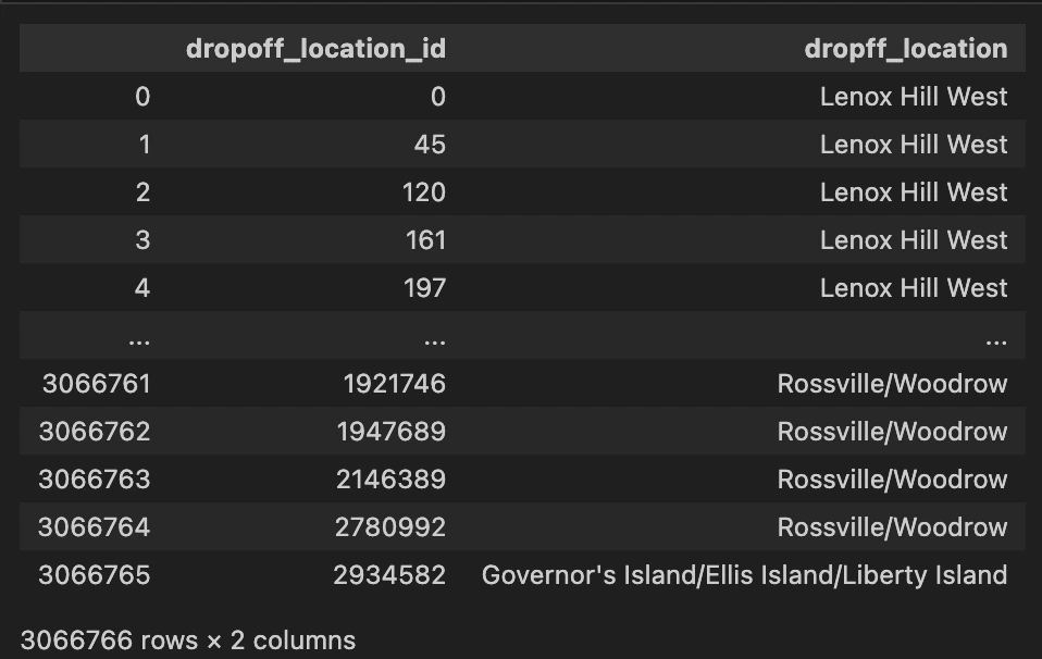
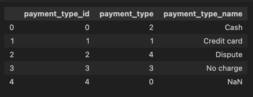
Creating payment_type_dim dimension table
payment_type_dim dimension tableAgain, if we look in the data dictionary the information about payment_type is provided e.g 1 = 'Credit Card' etc. This would be helpful for analysts when making complex join on data for analytical purposes
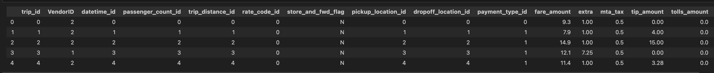
Creating fact_table dimension table
fact_table dimension tableThe most important table, where all of the data gets connected. This table doesn't hold descriptive information about the items themselves or the customers—instead, it links to other tables (like dimensions) that contain this additional information. So, while the fact table holds the numeric facts or measurements, it references other tables to provide the context or details about those facts. think of a fact table as the central hub of a data warehouse or database. It's where all the key metrics and measurements are stored, organized, and connected.
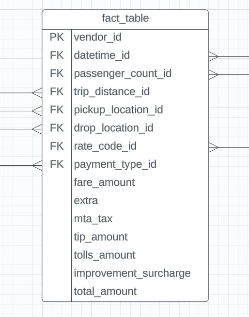
as we can see the table contains foreign keys of the dimension table and it represent a consolidated table which can link different tables to get different information of the trips.
Applying Analytics
What good a data model is when we can't apply analytics to it. I have prepared some questions in advance that we can answer. I will be using DuckDB for this exercise but in future articles (i hope :v ) i will be utilising clickhouse.
Basic Statistics:
What is the average trip distance?
What is the most common payment type?
Average trip distance for trips with a tip_amount greater than $10, excluding trips with a payment type of 'Cash'.
Vendor Comparison:
How many trips were made by each VendorID?
Which vendor has the highest average fare_amount?
Time Analysis:
What is the average number of passengers for trips that occurred on Sundays?
What are the peak hours for taxi trips based on the pick-up datetime?
Location-Based Analysis:
identify zones with the highest average total_amount and the lowest average trip_distance.
Which pickup location has the highest tip_amount amount?
Rate Code Insights:
How many trips were made for each rate code type?
What is the average total_amount for each rate code type?
Variables:
The pandas variables which holds information about dimensions
datetime_dim: This table captures datetime-related attributes such as pickup and drop-off hours, days, months, years, and weekdays.
passenger_count_dim: Contains passenger count information.
trip_distance_dim: Holds details about trip distances.
rate_code_dim: Provides insights into different rate codes and their corresponding names.
location_dim: A look-up table for location which maps locationID for pickup/dropff into location_name
pickup_location_dim: Stores data about pickup locations.
dropoff_location_dim: Holds data regarding drop-off locations.
payment_type_dim: Contains information about various payment types.
fact_table: Info about all relation to dimensions
I will create a helper function
Answering Basic Statistics Questions
Vendor Comparison:
How many trips were made by each VendorID?
Which vendor has the highest average fare_amount?
Time Analysis:
What is the average number of passengers for trips that occurred on Sundays?
What are the peak hours for taxi trips based on the pick-up datetime?
Location-Based Analysis:
identify zones with the highest average total_amount and the lowest average trip_distance.
Which pickup location has the highest tip_amount amount?
Rate Code Insights:
How many trips were made for each rate code type?
What is the average total_amount for each rate code type?
Like this project
Posted Jan 12, 2024
A Complete Data Engineering Workflow, Data Modelling and Advanced Analytics using Python, DuckDB - GitHub - DanielOX/Data-Engineering-Workflow-DUCKDB: A Comple…