You Can Save a Lot of Money on Health Insurance, But...

Ryhannul Jannah

Data Visualizer

Data Analyst

Statistician

Tableau

The high cost of treating COVID-19 has made many realize that health insurance is essential, especially during a pandemic. The pandemic has made many people feel their health and lives are in danger.

This conclusion emerged from a research of Inventure Indonesia with the Alvara Research Center on November 2020, which shows that 78.7% of respondents agreed that one needs health insurance hence the pandemic.

I conducted this exploratory on a Dataset from Medical Insurance Pay-out | Kaggle about individual total healthcare charges from ACME Insurance Inc., an insurance provider company that offers affordable health insurance to thousands of customers in the United States. It contains 1,338 records of data with six attributes excluding the Total Charge.

Fun Fact McKinsey’s benchmarking in the European retail trade has shown that the economic impact of intensive data evaluation is around three times higher in the insurance sector.

Part 1: Statistical Descriptive Analysis

The process begins with the essential thing, summarizing the attributes, such as finding the average & data distribution. Here I will break down all the attributes to ease understanding of the data set.

Attribute #1 : Age

There is a growing risk of disease as humans age. In most cases among humans, aging leads to a gradual decrease in physical and mental capacity. This is the impact of accumulating a wide variety of molecular and cellular damage over time (WHO, 2022). In most states, age is one factor in determining individual medical insurance rates.

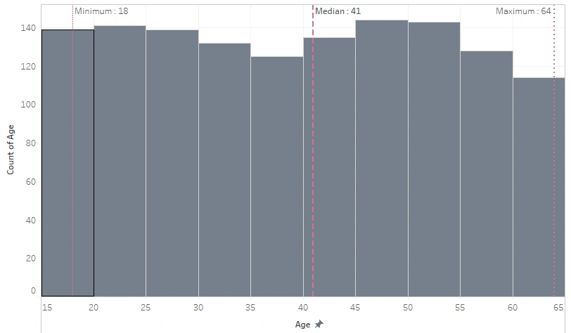
Distribution of Age

The Median for age of beneficiaries is 41 years old; the youngest is 18 years old, and the oldest is 64.

In the United States, seniors over 65 already get healthcare coverage from Medicare, so they do not need private insurance. Kids under 26 practically do not need private health insurance as well because, since 2010, the regulation in the US states that their parent’s insurance plan automatically protects them without any condition (Dowshen, 2018).

Regarding the existence of a lot of data age 25-and-below here, I assume the health insurance package taken by their parents is insufficient to cover them, or perhaps they don’t have anybody’s insurance to protect them. Another possibility is they probably got the insurance before the law took effect.

Attribute #2 : Sex (Binary)

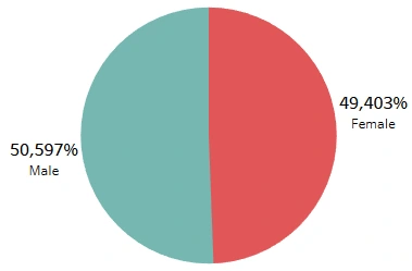
Proportion of Sex

The proportion of male and female beneficiaries in the data is almost equal.

Attribute #3 : Region (US Residential Area)

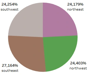
Proportion of Each Region

The distribution of beneficiaries is sequentially the highest in the Southeast, Northwest, Southwest, then Northeast. More than a quarter of the sample lives in the Southeast, about 2.6% more than in the Northwest. Whereas the other three areas only differed by about 1–1.5% one another.

Attribute #4 : Smoking Habit

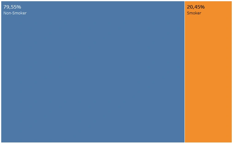
Proportion of Smoker vs Non-Smoker

In the data we use, only 20.45% or approximately one-fifth of the sample recorded as a smoker.

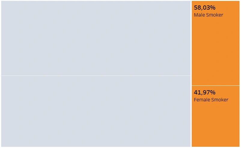
Sex Proportion of the Smoker

Broken down, the graph shows that there is a probability of 0.58 that a smoker is a male (and 0.42 of a female).

Attribute #5 : Body Mass Index (BMI)

BMI expresses the relationship between height and weight as a single number without depending on frame size. In general, the higher your BMI, the higher the risk of developing a range of conditions linked with excess weight. Nearly three million people die yearly from being overweight or obese, according to WHO.

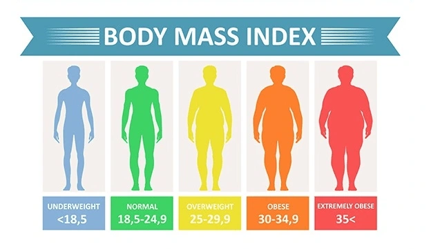
BMI Classification (Source: palingmales.com)

BMI classification states that a standard BMI ranges between 18.5 and 25; a range of 25 to 30 is considered overweight, and BMI over 30 is considered obese. Conversely, a person is classified as underweight if the BMI is less than 18.5.

As BMI indicates your health and fitness levels, it affects your insurance premiums. The further from ‘normal’ BMI, the more hospital visits will occur, leading to more medical expenses, meaning a higher insurance premium. So the higher the projected costs for your health problems, the higher will be your insurance premium.

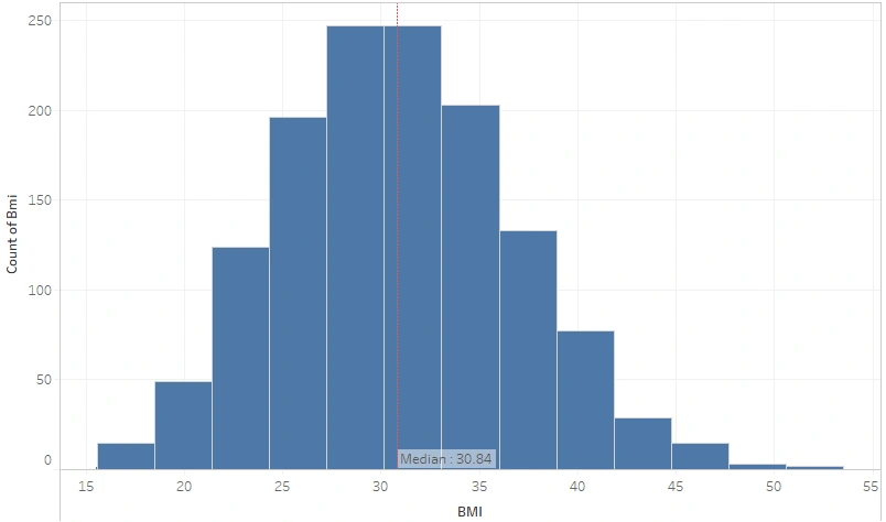
BMI Distribution

In this Dataset, the BMI data distribution is normal. The median BMI of all beneficiaries is 30.84 (Obese). Would there be any differences in the BMI of smokers and non?

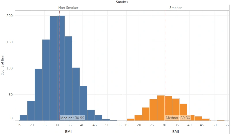
BMI Distribution by Smoking Habit

Both smokers and non-smokers are still obese-classified, but the non-smokers are 0.63 points better.

It is a widespread belief that smoking is an efficient way to control body weight. Biologically, tobacco use could increase the metabolic rate, decrease metabolic efficiency, or decrease caloric absorption (reduction in appetite), leading to weight loss. That metabolic effect of smoking could explain the lower body weight in regular smokers. However, why doesn’t the graph above show a significant difference?

A study shows that tobacco consumption is in line with other risk behaviors known to favor weight gain such as poor diet and low physical activity, especially in persons of lower socioeconomic status. These factors could counterbalance and even overtake the slimming effect of smoking. Another research also proves that weight cycling may be involved in the association between smoking and obesity, which could explain why smokers are also likely to be overweight or obese. Out of curiosity, let’s break it down into sex-wise.

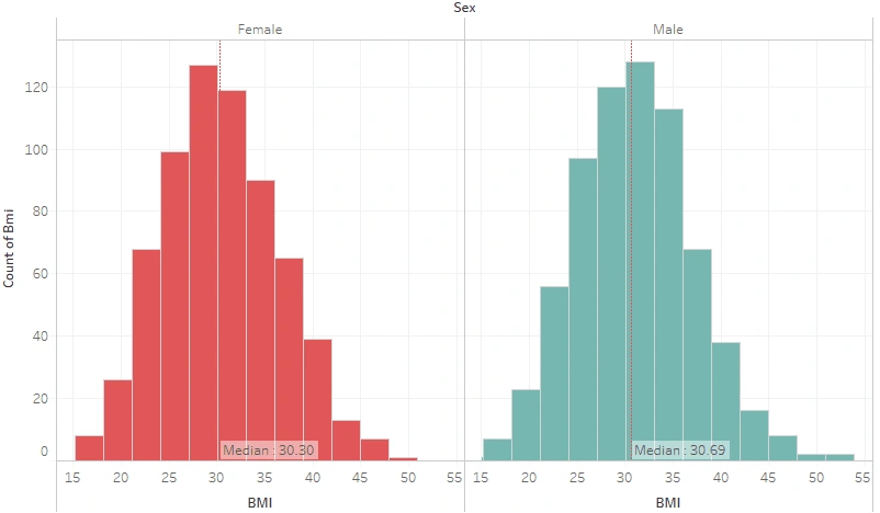
BMI Distribution by Sex

Females averagely have a lower BMI. There is a well-known theory that women’s BMI is naturally slightly lower than males because they are generally shorter in height, which means that the graph is actually in accordance with the theory. What if the condition is narrowed down to women and men who smoke?

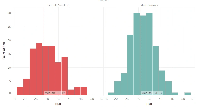
BMI Distribution of Male and Female Smokers

In addition to the fact that women’s BMI tends to be slightly lower than men’s BMI, A 2010 study also showed that males were significantly more often heavy smokers than females, except for those females who started smoking at an early age. These may explain why the BMI of female smokers is quite far lower than the BMI of male smokers. Even the BMI of female smokers is classified better (overweight). To close this session, let’s view the average BMI per region.

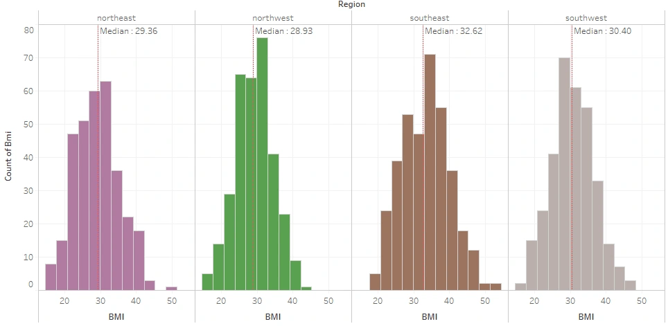
BMI Distribution per Region

The plot found that the average BMI of the insured living in the North was classified as severely overweight, with the Northwest still better than the Northeast. Meanwhile, the Southwest is mildly obese, while the Southeast is moderately obese.

The insured who live in the South are classified as obese, as is commonly known. Traditional Southern diet — high in fat and fried food — may be part of the reason why they have a high rate of Obese, said Dr. William Dietz, head of the Nutrition, Physical Activity, and Obesity division in the Centers for Disease Control and Prevention. The South also has a large concentration of rural residents and black women — two groups that tend to have higher obesity rates, he said.

The proportion of each binary sex in this dataset is nearly equal, with an (almost) uniform age distribution range of 18–64 years old.

Overall, one in five insureds has a smoking habit, with about 60% of the smokers being Male. Male and Female smokers detach regarding BMI classification; female smokers tend to be Overweight whilst male smokers are Obese. Region-wise, the West is Overweight while the East is Obese with the Southeast being the worst.

Part 2: Variable Analysis

Here we are going to determine the probability that a particular condition has the potential to have a certain amount of medical charges.

As the main concern, let’s plot the medical charges first.

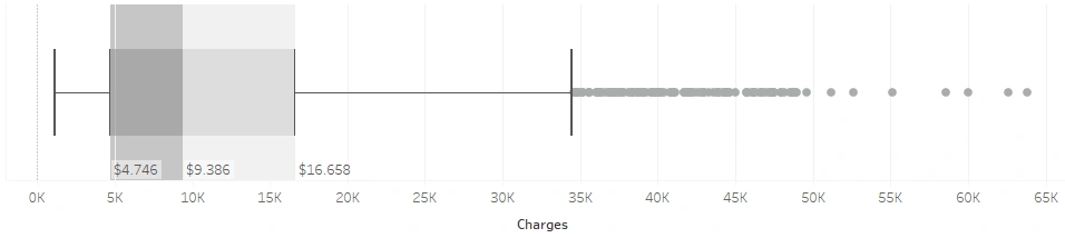
The distribution of medical charges is positively skewed, with a median of $9,386. The densest spread of total bills is in the range of $4,746 — $ 9,386 while the median of the upper half is $16,658. At a glance, it appears that the beneficiary data cluster into two: cluster 1 consists of beneficiaries with a total bill of less than $15,000, and cluster 2 is a total bill of more than $15,000. Let’s break this down into several conditions.

Which sex has the higher total pay-out, male or female?

This is subjectively an interesting one for me. On one side, I assume that women have higher bills because childbirth is one of the highest healthcare costs. Yet on the other hand, in addition to having more smokers, many men also have activities or jobs in rough fields which might harm them fatally. It turns out that:

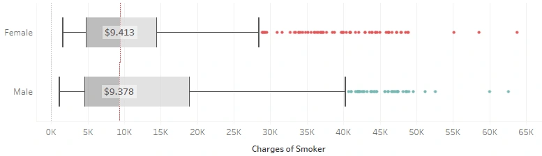
in general, both males and females have a median total bill that is nearly the same even though both have many outliers. Both distributions are also positively skewed.

The difference we can notice between them lies in the skewness. The data on males extends to $40k while the female reaches only around $28.5k. The farther upper hinge and the more prolonged upper whisker for males mean more males have to pay above the average beneficiaries than females, yet in general, males’ bills are (slightly) lower than females’ bills.

Does above-normal BMI result in a higher charge?

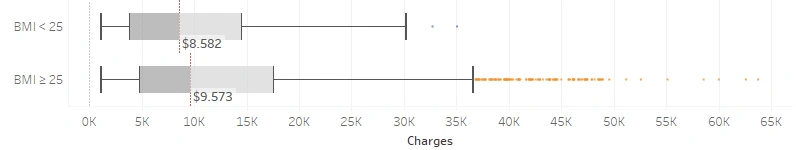
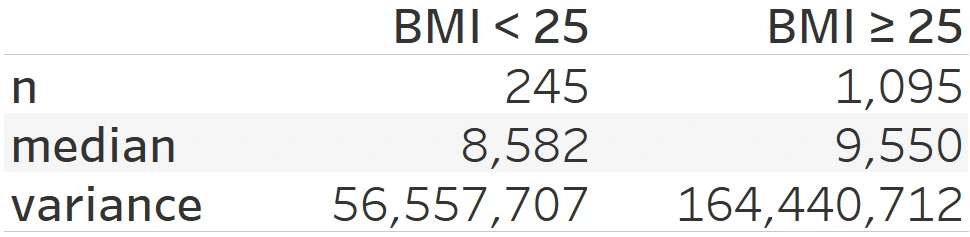
The insured with above-normal BMI (BMI≥25) have a higher bill and more considerable data variance. The difference is about $1000. Outliers in the BMI≥25 is also shown to be quite extreme, in contrast to BMI<25.

Having a lower BMI, is the charge of the Northerns cheaper than the Southern?

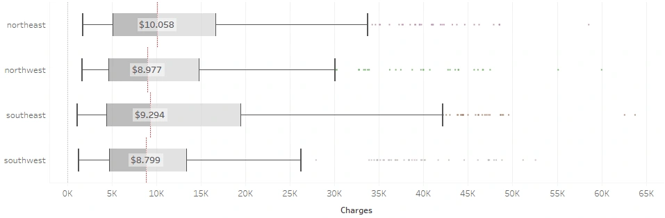
Southwest residents have the lowest bills, while Northeast residents tend to have the highest. The four regions practically have average bills that are similar, but it turns out that the average total charge doesn’t diverge into North vs. South, yet East vs West. Wests’ are slightly cheaper with both coming in at less than $9k on average, while Easts’ are over $9k on average. A specific condition must have caused this, perhaps, the smokers’ proportion?

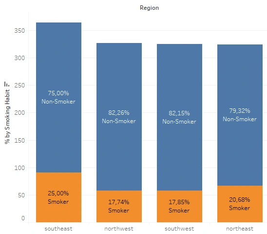
Both Easterns have more than 20% smokers which may be the cause of considerable medical charge data variance and median in both, whereas Westerns have less than 18% smokers in theirs. Moreover, Southwest is well known for its pleasant temperature. An article says that their summer tends to be warm and sunny, making it easier to go out and be active. Complementarily, the winter is also mild and tolerable; the roads are still travel-safe, while outdoor activities and exercise are still easy to maintain.

In addition to that, Moneygeeks also stated that the overall affordability of healthcare in the Northeast is indeed the worst, while Southwest has the best one. So probably, Southwest can have the lowest total medical pay-out because of its healthier climate and lifestyle along with the affordable healthcare costs.

May I say that the smoking habit causes a higher charge?

Part 1 noted that the proportion of smokers only takes up one-fifth of the total sample. With that small ratio, is the average health bill of smokers smaller than that of non-smokers?

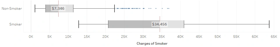
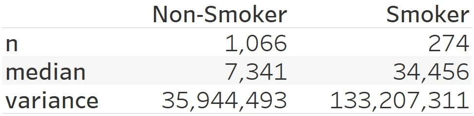
The central tendency of charge for the non-smokers is $7,346 with a variance of $35,944,493 while for the smoker is $34,456 with a variance of $133,207,311. The average charge for smokers is almost five times higher than that of non-smokers, they also produce a wider variance of data. Non-smokers generally get bills in the middle to lower nominal range, while the bill range for smokers is in the middle to the upper. To be calculated, the average charge for non-smokers is in the range of $1,350 to $13,336 while for the smoker is $22,914 to $45,997.

Interesting, isn’t it? There is only one-fifth of the people that smokes, but this one-fifth makes an average total bill up to five times compared to the other four-fifths. Truly a Pareto business.

However, although the distribution says so, the outliers somehow tell that non-smokers may still get a higher total bill than the average smoker. A study in 1997 shows that non-smokers tend to live longer; thus, they will reach old age when the chance of their health problems increases as they age and incurs more costs due to those diseases, particularly in old age when the prices are highest. Smokers are one contributor to the high average medical bill.

What if we compare only females and males who smoke?

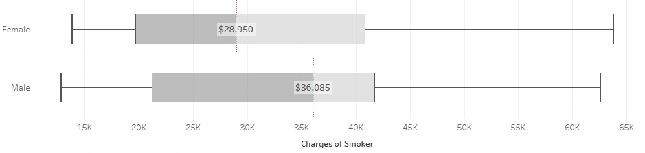
Apparently, the two distributions are pretty similar in distribution, but the median is quite far apart. The median of male smokers was $36,085 while that of female smokers was $28,950. Males do have a higher total charge than females when given that they smoke.

Up to this point, it has been identified that the smoking habit is a contributor that needs to be taken into account in determining medical insurance premiums. However, bills for male smokers are higher than for female smokers.

With male smokers having a higher BMI, does the combination of smoking and a high BMI mean a higher bill? I am going to break this down below.

What is the correlation between BMI and Smoking Habit to Medical Charges?

Here, I first plotted between BMI and Bills to see the correlation.

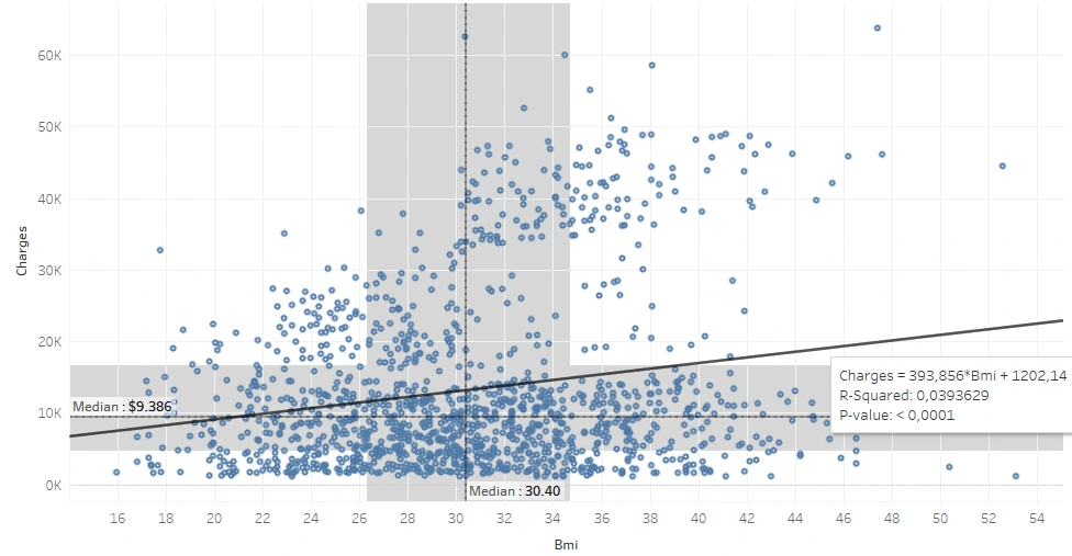
BMI and charge are shown as positively correlated, but the correlation value is too small (0.198) to declare a correlation between each other. The trend line shows that for every 0.1 BMI increase, there is an increase in the total bill of $39. We can see at a glance that the population seems divided into two, we’ll look into it later.

I tried to plot the cumulative distribution function (CDF) to see how big the chance is that someone classified as overweight or above (BMI ≥ 25) to get a medical bill above the average or even exceed the upper quartile ($16,700).

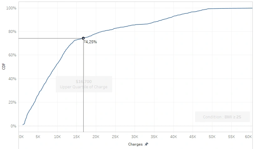
Only 25.75% people with BMI ≥ 25 billed more than the upper quartile, while those more than the median reached 50.78%. Half of them got above-average bills and the other half didn’t. Thus, BMI does not necessarily correlate with the amount of health bills. Thereupon, I separated the data based on smoking habits by coloring the dots differently.

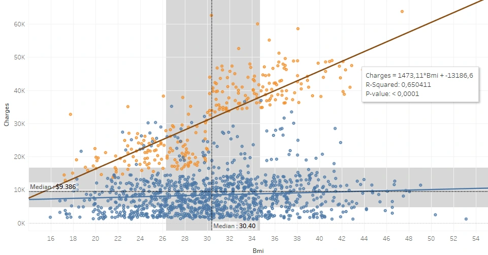
In the plot above, the yellow dots indicate smokers. Here it is clear that a robust correlation exists between BMI and the total bill of smokers. For every 0.1 increase in a smoker’s BMI, the total bill adds $147. There is no significant correlation coefficient in the non-smoker data.

All the yellow dots appear to be consistently above the blue dots even though some of the blue dots are isolated in the area of the yellow, meaning that, in general, smokers have higher bills than non-smokers.

I tried to plot the CDF to calculate the probability that smokers will get a bill that exceeds the upper quartile, regardless of their BMI score.

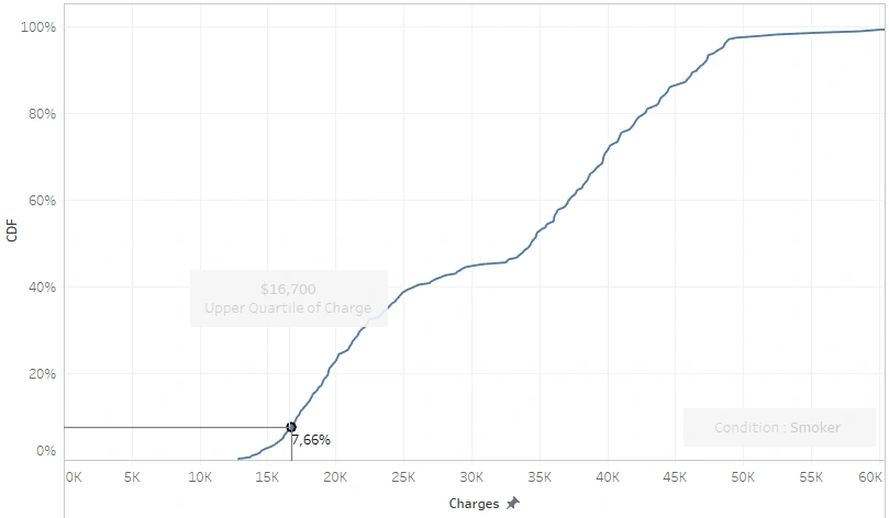
7.66% of smokers’ bills are below the upper quartile, meaning that 92% of them billed more than $16,700; let alone those exceeding the median.

Another thing we can see in the last scatter plot is that there are two populations of smokers, a BMI below 30 (under-Obese) and a BMI above 30 (Obese). The bills of obese smokers are well over $30,000, meaning that their statements are sure to exceed the upper quartile of the entire population, while for a smoker whose BMI is under-obese:

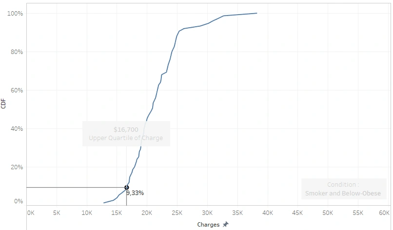
they have a probability of 0.9 to get a medical insurance pay-out of more than $16,700 and a 50:50 chance of being billed for more than (or less than) $21,000.

Part 3: Statistical Hypothesis Test

All the plotting results up there need to be statistically proven. This part will show steps for finding statistical evidence on several identifications mentioned above. I am going to use a 5% significance level toward 1,338 data samples in the following tests.

Test #1 : Males’ health bills are lower

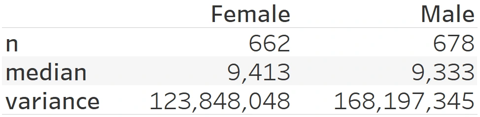
Step 1 – Two Variance Test

Since male has a higher variance, it will be used as the numerator (m) while the other one is the denominator (f). The hypothesis of this test would be:

H0: σ²m = σ²f→ the variance of m is equal to the variance of f H1: σ²m ≠ σ²f→ the variance of m is not equal to the variance of f

With a degree of freedom of 677 for Males and 661 for females, the critical F-value is calculated at 1.136 by Online Calculator. Next, we need to calculate the F-test by dividing the larger variance value to the smaller variance value.

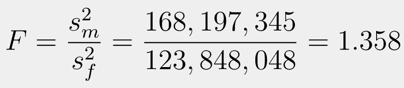
It shows that the F-value is higher than the critical F-value, so H0 is rejected at the 0.05 significance level because F>1.136 (F=1.358). Since there is no evidence that males’ and females’ variance is the same, then the variances are not equal.

Step 2 – T-Test of Two Samples

H0: 𝜇Males’ Bills ≥ 𝜇Females’ Bills H1: 𝜇Males’ Bills < 𝜇Females’ Bills

We will perform a lower-tailed t-test because we need to test the mean of two samples, while we don’t have any information about the population’s standard deviation. To do the test, we need to calculate the Degree of Freedom which we will then use in calculating the critical t-value.

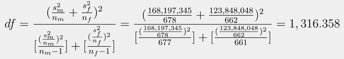
Here obtained 1,316.358 degrees of freedom. Since Degree of Freedom >1000, I will test the p-value towards the significance level (0.05) instead of the t-value of the critical t-value. Next, I am going to calculate the t-score for unequal variances.

We have got the Degree of Freedom and t-value; now, we calculate the p-value using an online calculator. It was calculated that the p-value is 0.495.

Finally, it turns out that the p-value is not statistically significant. In the assumption that the males’ bill ≤ females’ bill, we will get a sample of males’ bills > females’ bills in 49% of observations with 0,05 level of significance; then there is not enough evidence to reject H0 so that H0 is accepted (Males’ Bills ≥ Females’ Bills)

Test #2 : BMI≥25 Gets Higher Charge

This part will challenge the claim that ‘BMI-Overweight (or more) have a higher medical charge.’ Again, we need to test first whether both variances are the same.

Step 1 — Two Variance Test

Since it has a higher variance, the BMI≥25 will be used as the numerator (x) while the other one is the denominator (y). The hypothesis of this test would be:

H0: σ²x = σ²y → the variance of x is equal to the variance of y H1: σ²x ≠ σ²y → the variance of x is not equal to the variance of y

Knowing that the degree of freedom of x is 1,094 and the degree of freedom of y is 244, then obtained the critical F-value is 1.185. Next, we calculate the F-test by dividing the larger variance value to the smaller variance value.

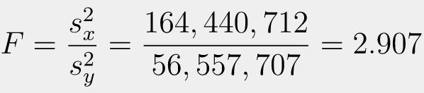
The F-value is higher than the critical F-value, so H0 is rejected at the 0.05 significance level because F>1.185 (F=2.907). Since there is no evidence that the variance of the data on BMI≥25 and BMI<25 is the same, the variances are not equal.

Step 2 — t-Test of Two Samples

H0: 𝜇(BMI≥25) ≤ 𝜇(BMI<25) H1: 𝜇(BMI≥25) > 𝜇(BMI<25)

We are going to use the t-test (again) since we need to perform a mean test without getting the information on the population standard deviation. We need to calculate the Degree of Freedom (df) — as usual — to be able to get the critical t-value.

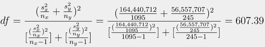
Here obtained 607.39 degrees of freedom, so this upper tail testing has a critical t-value of 1.647, meaning H0 will be rejected when t>1.647 (or the p-value<0.05).

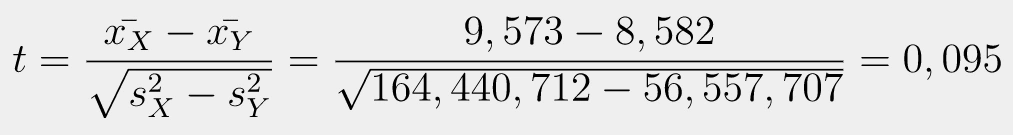
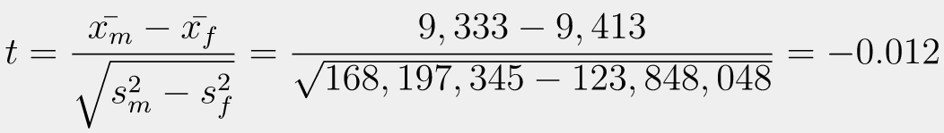
The equation above shows the outcome of the t-test calculation. Obtained that H0 is accepted; We have statistically significant evidence at a significance level of 0,05 to show that the medical charge of BMI≥25 is not proven to be higher than BMI<25 because t<1.647 (t=0,095).

Test #3 : Smokers’ Medical Bills are Higher

Before testing the average of the two samples, we will conduct F-test to see whether the variances of both conditions are the same.

Step 1 – Two Variance Test

The smoker has a higher variance so it is going to be the numerator (sm) while the other one is the denominator (ns). The hypothesis of this test would be:

H0: σ²sm = σ²ns → the variance of sm is equal to the variance of ns H1: σ²sm ≠ σ²ns → the variance of sm is not equal to the variance of ns

With a degree of freedom of sm is 1,065 and the degree of freedom of ns is 273, the critical F-value is calculated at 1.176. Next, we need to calculate the F-test by dividing the larger variance value to the smaller variance value.

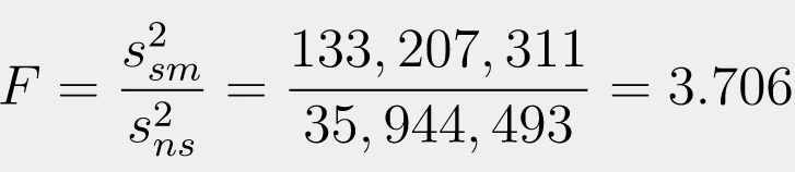
The calculation shows that the F-value is higher than the critical F-value, so H0 is rejected at the 0.05 significance level because F>1.176 (F=3.706). Since there is no evidence that the variance of the data on smokers and non-smokers is the same, the variances are not equal.

Step 2 – T-Test of Two Samples

H0: 𝜇Smokers’ Bills ≤ 𝜇Non-Smokers’ Bills H1: 𝜇Smokers’ Bills > 𝜇Non-Smokers’ Bills

We are going to use the t-test since we need to perform a mean test without getting the information on the population standard deviation. We need to calculate the Degree of Freedom (df) to be able to get the critical t-value.

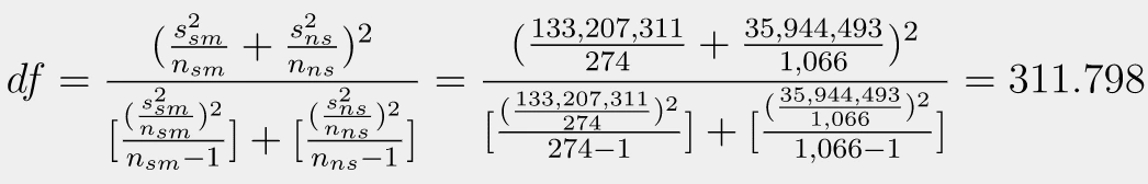
Here obtained 311.8 degrees of freedom, so this upper tail testing has a critical t-value of 1.65 calculated by an online calculator, meaning H0 will be rejected when t>1.65 (or the p-value<0.05).

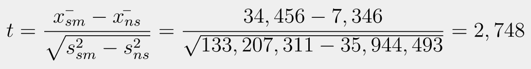
The equation above shows the outcome of the t-test calculation for unequal variances. Since we got no evidence that the bill of smokers is the same as that of non-smokers, then H0 is rejected; the medical charge of smokers proved to be higher than non-smokers with a significance level (0.05) because t>1.65 (t=2.748).

SUMMARY

All the analyses show that gender and smoking habits influence the number of medical charges. At the same time, a high BMI independently has not been proven to have anything to do with a higher bill.

Males’ bills are higher or equal to females’; there is not enough evidence to reject that.

BMI-classified as Overweight, Obese, or Extremely Obese (alone), does not guarantee that one’s will have a higher bill than those whose BMI is Normal or Underweight.

Smoking habit produces a higher bill.

you can save a lot of money on medical insurance, but you smoke. in short, don’t 🤷🏻‍♂️

Like this project

Posted Sep 30, 2024

US citizens tend to fall into the BMI classification of obesity. It might sound stereotyping but the data says so...

Likes

Views