Breast Cancer Diagnosis Classification Using Naive Bayes

Preprocessing Data

1. Data Information: Use the `info()` function to obtain information about the number of entries and data types in each column.

2. Data Description: Use the `describe()` function to understand the distribution of values in each feature.

3. Histogram Visualization: Visualize the distribution of each feature using histograms.

4. Null Values: Check for null values using the `isnull()` and `sum()` functions.

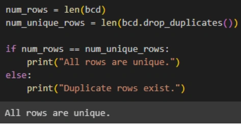
5. Duplicate Rows: Check for duplicate rows using the `duplicated()` function and remove them if found.

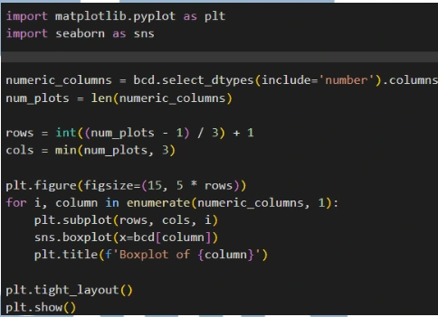
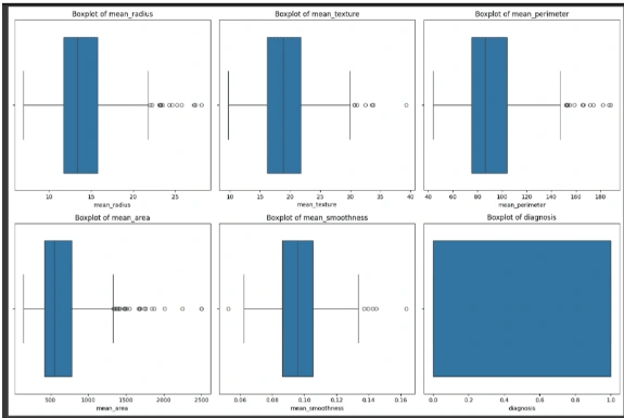
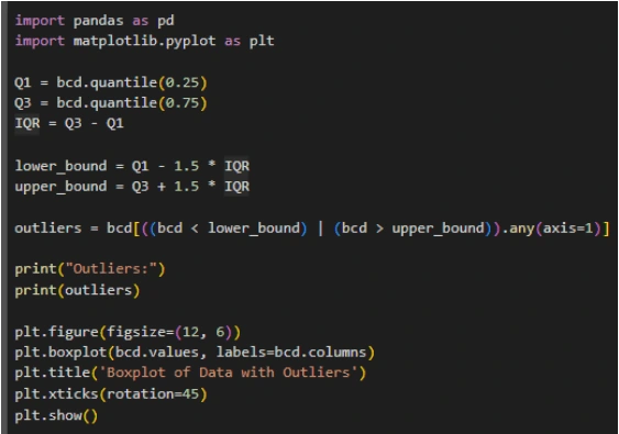
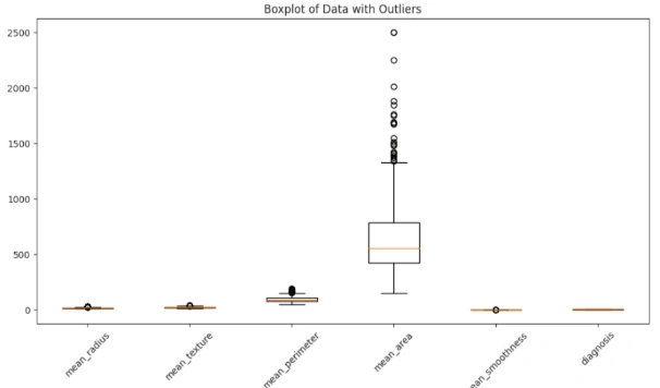
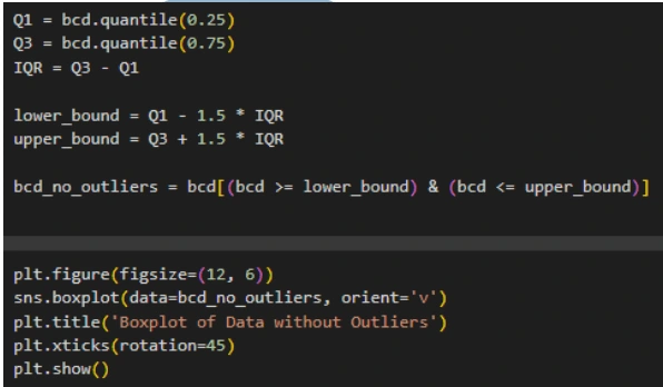
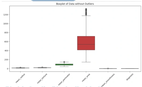
6. Outliers: Identify outliers using the interquartile range (IQR) method and visualize the data with and without outliers using boxplots.

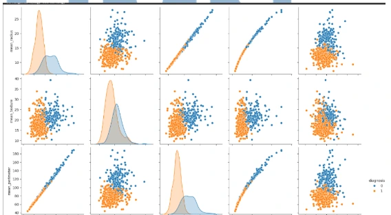
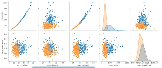
7. Feature Distribution: Identify the distribution of certain numerical features using histograms.

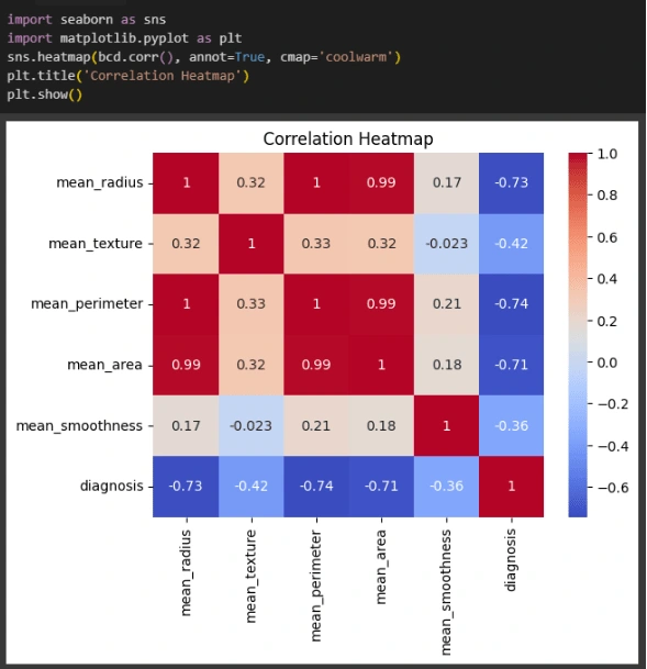
Feature Engineering

1. Data Description: Use the `describe()` function to obtain descriptive statistics such as mean, median, and quartiles for each feature.

2. Histogram Visualization: Visualize the distribution of each feature using histograms with the `histplot()` function and the seaborn library.

3. Outlier Detection: Identify and handle outliers in the dataset using the IQR method.

4. Goal: The goal of feature engineering is to improve data quality and prepare the dataset for classification using the Gaussian Naive Bayes algorithm.

Data Split

1. Splitting Dataset: Use the `train_test_split()` function from the scikit-learn library to split the dataset into training and test sets.

2. Training and Testing: Allocate 70% of the data for training and 30% for testing.

3. Random State: Use `random_state=42` to ensure reproducibility of the results.

Modeling Data

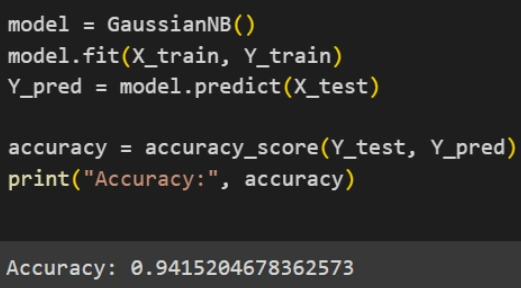
1. Initialization: Initialize the Gaussian Naive Bayes model using `GaussianNB()` from the scikit-learn library.

2. Training: Train the model using the training data with the `fit()` method.

3. Prediction: Use the trained model to make predictions on the test data with the `predict()` method.

4. Evaluation: Evaluate the model's performance using metrics such as accuracy and confusion matrices.

Validation and Evaluation

1. Data Split: Split the dataset into training and test sets using `train_test_split()` from the scikit-learn library.

2. Training: Train the Gaussian Naive Bayes model using the training data.

3. Prediction: Make predictions on the test data using the trained model.

4. Evaluation Metrics: Evaluate the model's performance using metrics such as precision, recall, and F1 score.

5. Visualization: Visualize the decision boundaries and probability predictions using `plot_decision_boundaries()` and `plot_probabilities()`, respectively.

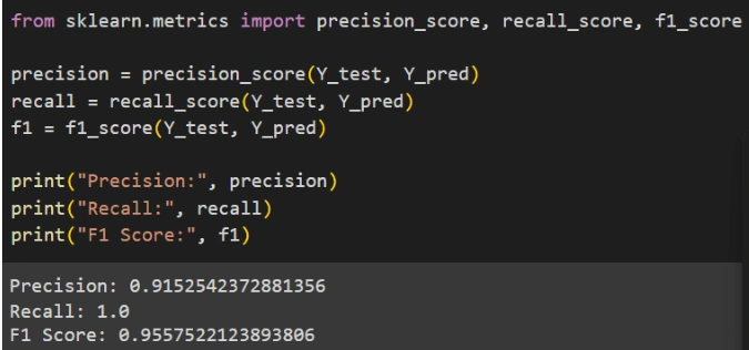
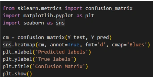
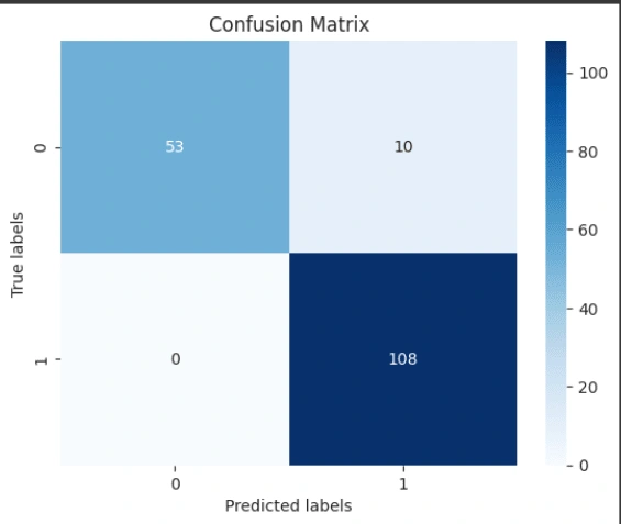
Based on the evaluation results, it can be concluded that the Gaussian Naive Bayes model performs well in predicting test data and shows consistent results in cross-validation. The model has an accuracy of 94.15%, indicating that it can accurately predict around 94.15% of the test data. Additionally, the model has a precision of 91.53%, meaning that 91.53% of all positive predictions made by the model are indeed positive. The recall of the model reaches 100%, showing that it successfully detects all positive instances in the dataset without missing any. The F1 score of the model is 95.58%, which is a combination of precision and recall, indicating a good balance between the two. The cross-validation results show that the average accuracy of five cross-validation runs is around 89.28%, which is slightly lower than the accuracy on the test data but still indicates good and consistent performance. Overall, the Gaussian Naive Bayes model shows high performance with good accuracy and a balance between precision and recall, as well as consistent results from cross-validation, making it a good model for classification in this case.