Renting prices in Algeria (Data scraping, EDA, ML)
Youcef Belmokhtar
In [231]:
import matplotlib.pyplot as plt
import seaborn as sns
Renting price in Algeria

Today, I'm gonna make some analsyis on Renting price in Algeria (my country). I'm gonna scrap the data from an Algerian website, process it, make some analysis then try to build a machine learning model to predict the Final renting price.

Scapped data will be used for learning purpose only, no commercial use!
Data Scraping:
In [2]:
from urllib.request import urlopen
from bs4 import BeautifulSoup
import re
import requests
In [24]:
title=[]location=[]size=[]agence=[]price=[]detail=[]
In [23]:
details=soup.find_all('ul',class_="listing-details")
In [25]:
url='https://darjadida.com/annonces/immobilier?q=location+appartement&per_page='for z in range(1,100): html = requests.get(url+str(z)) soup= BeautifulSoup(html.content,'lxml') titles=soup.find_all('h4') locations=soup.find_all('a',class_="listing-address popup-gmaps") sizes=soup.find_all(class_="listing-details") agences=soup.find_all('div',class_="listing-footer") prices=soup.find_all('span',class_="listing-price") details=soup.find_all('ul',class_="listing-details") for i in range(len(details)): title.append(titles[i].text) location.append(locations[i].text) agence.append(agences[i].text) price.append(prices[i].text) detail.append(details[i].text)
In [82]:
data=[title,detail,location,size,agence,price]
In [83]:
dict={'titre':title,'detail':detail,'local':location,'vendeur':agence,'prix':price}
In [84]:
df = pd.DataFrame(dict)
Data Cleansing:
In [85]:
df['detail']=df['detail'].str.replace('\n','')df['detail']=df['detail'].str.strip()
In [86]:
df.loc[df['detail'].str.contains('F1'), 'Type'] = 'F1'df.loc[df['detail'].str.contains('F2'), 'Type'] = 'F2'df.loc[df['detail'].str.contains('F3'), 'Type'] = 'F3'df.loc[df['detail'].str.contains('F4'), 'Type'] = 'F4'df.loc[df['detail'].str.contains('F5'), 'Type'] = 'F5'df.loc[df['detail'].str.contains('F6'), 'Type'] = 'F6'
In [87]:
df['Bedrooms']=df['Type'].str[1:2]df['City']=df['titre'].str[24:]df['M²']=df['detail'].str[4:8]df=df.dropna()
In [102]:
df.loc[df['titre'].str.contains('Bejaia'), 'City'] = 'Bejaia'df.loc[df['titre'].str.contains('Annaba'), 'City'] = 'Annaba'df.loc[df['titre'].str.contains('Bouira'), 'City'] = 'Bouira'df.loc[df['titre'].str.contains('Alger'), 'City'] = 'Alger'df.loc[df['titre'].str.contains('Tizi-ouzou'), 'City'] = 'Tizi-ouzou'df.loc[df['titre'].str.contains('Constantine'), 'City'] = 'Constantine'
In [115]:
df=df.drop(columns=['titre','detail','Type','size'],axis=1)
In [122]:
df=df.drop(columns='local',axis=1)
In [124]:
df.loc[df['prix'].str.contains('DA'), 'Is there a price?'] = 'Yes'
In [126]:
df=df.dropna()
In [128]:
df=df.drop(columns='Is there a price?',axis=1)
In [132]:
df['Price']=df['prix'].str[:8]
In [134]:
df=df.drop(columns='prix',axis=1)
In [137]:
df['vendeur']=df['vendeur'].str.replace('\n','')df['vendeur']=df['vendeur'].str.strip()
In [151]:
df['Agency']=df['vendeur'].str[:-10]
In [153]:
df=df.drop(columns='vendeur',axis=1)
In [ ]:
df['M²']=df['M²'].str.replace('M','')df['Price']=df['Price'].str.replace('D','')df['Price']=df['Price'].str.strip()df['Price']=df['Price'].str.replace(' ','')df['Price']=df['Price'].str.replace('A','')df['Price']=df['Price'].str.replace('.','')
In [194]:
df['Price']=df['Price'].astype('int')df['Bedrooms']=df['Bedrooms'].astype('int')
In [200]:
df['M²']=df['M²'].str.strip()df['M²']=df['M²'].str.replace('tudi','')df['M²']=df['M²'].str.replace('²','')
In [201]:
df['M²']=df['M²'][df['M²']!=''].astype('int')
In [209]:
df = df[['Bedrooms', 'M²', 'City', 'Agency','Price']]
In [213]:
df['City'].unique()
Out[213]:
array(['Alger', 'Tizi-ouzou', 'Bejaia', 'Boumerdes', 'Constantine', 'Jijel', 'Saida', 'Oran', 'an', 'Annaba', 'Borj-bou-arreridj', 'Blida', 'Biskra', 'Setif', 'Tipaza', 'Bouira', 'Mostaganem', 'Sidi-belabbes', 'Oum-elbouaghi', 'El-tarf'], dtype=object)
In [229]:
df = df[df.City != 'an']
In [433]:
plt.style.use('classic')
In [435]:
plt.style.use('Solarize_Light2')
Exploratory data analysis:
In [451]:
Price_per_city=pd.pivot_table(df,index='City',values='Price')Price_per_city=Price_per_city.sort_values(by='Price',ascending=False)Price_per_city=Price_per_city.head(5)Price_per_city.plot(kind='barh',figsize=(10,8),title='Most expensive cities',edgecolor='black')
Out[451]:
<AxesSubplot:title={'center':'Most expensive cities'}, ylabel='City'>
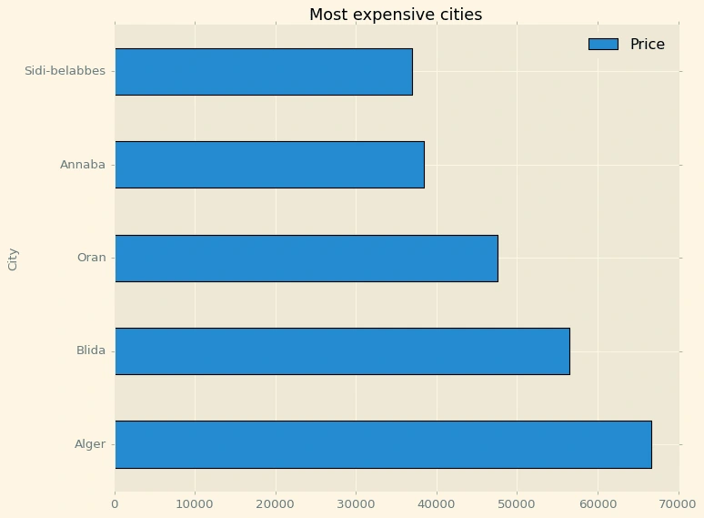
Alger, the capital, has the highest average renting price.
In [490]:
df['Price'].plot(kind='hist',bins=75,figsize=(12,7),edgecolor='black',title='Price distribution')
Out[490]:
<AxesSubplot:title={'center':'Price distribution'}, ylabel='Frequency'>
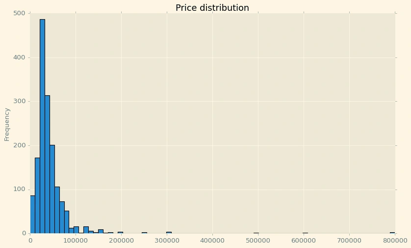
Most of renting prices range between 0-100000 DA
In [455]:
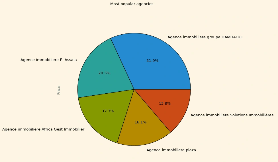
Agencycount=pd.pivot_table(df,index='Agency',values='Price',aggfunc='count')Agencycount=Agencycount.sort_values(by='Price',ascending=False)Agencycount=Agencycount[1:].head(5)Agencycount.plot(kind='pie',figsize=(8,8),subplots=True,autopct='%1.1f%%',title='Most popular agencies',legend=False)
Out[455]:
array([<AxesSubplot:ylabel='Price'>], dtype=object)
In [452]:
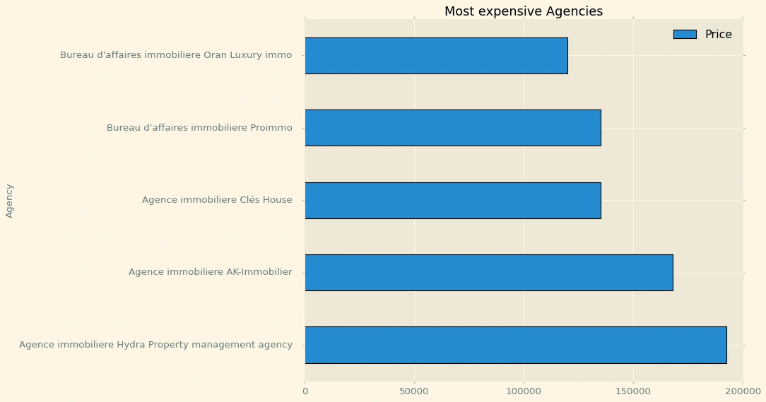
Agencyprice=pd.pivot_table(df,index='Agency',values='Price',aggfunc='mean')Agencyprice=Agencyprice.sort_values(by='Price',ascending=False)Agencyprice=Agencyprice.head(5)Agencyprice.plot(kind='barh',figsize=(10,8),title='Most expensive Agencies',edgecolor='black')
Out[452]:
<AxesSubplot:title={'center':'Most expensive Agencies'}, ylabel='Agency'>
In [453]:
Agencyprice=pd.pivot_table(df,index='City',values='Price',aggfunc='count')Agencyprice=Agencyprice.sort_values(by='Price',ascending=False)Agencyprice=Agencyprice.head(5)Agencyprice.plot(kind='bar',figsize=(10,8),title='Top 5 cities per count',edgecolor='black')
Out[453]:
<AxesSubplot:title={'center':'Top 5 cities per count'}, xlabel='City'>
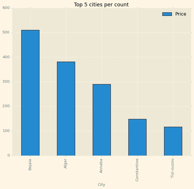
Bejaia has the highest available appartements.
In [489]:
Agencyprice=pd.pivot_table(df,index='City',values='M²',aggfunc='mean')Agencyprice=Agencyprice.sort_values(by='M²',ascending=False)Agencyprice=Agencyprice.head(5)Agencyprice.plot(kind='bar',figsize=(10,8),title='Top 5 cities per Area',edgecolor='black')
Out[489]:
<AxesSubplot:title={'center':'Top 5 cities per Area'}, xlabel='City'>
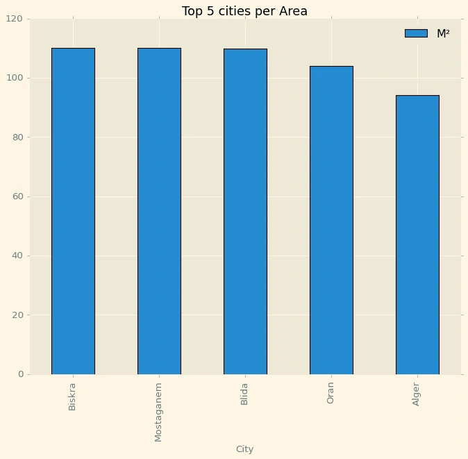
They are almost equal
In [465]:
ddd=df[['Bedrooms','Price']].groupby('Bedrooms').mean()ddd.plot(kind='line',color='b',title='Average Price per number of bedrooms')
Out[465]:
<AxesSubplot:title={'center':'Average Price per number of bedrooms'}, xlabel='Bedrooms'>
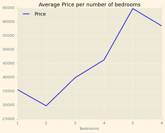
Price will increase with number of bedrooms
In [483]:
ddd1=df[['M²','Price']].groupby('M²').mean()ddd1.plot(color='b',title='Average Price per M²',figsize=(12,6))
Out[483]:
<AxesSubplot:title={'center':'Average Price per M²'}, xlabel='M²'>
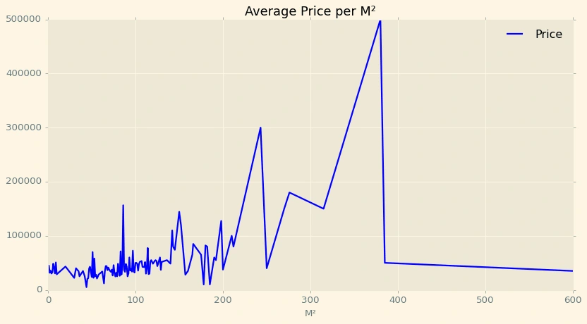
In general, Price increase when the area increase
In [421]:
df2=df.copy()
In [422]:
df2=df2.dropna()
In [423]:
df2['City']=pd.factorize(df2.City)[0]df2['Agency']=pd.factorize(df2.Agency)[0]df2['Bedrooms']=pd.factorize(df2.City)[0]
In [424]:
df2['M²']=df2['M²'].fillna(81.17)
In [429]:
df2.head()
Out[429]:
BedroomsM²CityAgencyPrice1080.000013000031157.0011280005265.00203000073120.0032500009089.000390000
Data correlation:
In [428]:
plt.figure(figsize=(12,8))sns.heatmap(df2.corr(),annot = True, cmap= 'YlGnBu', fmt= '.2f')
Out[428]:
<AxesSubplot:>
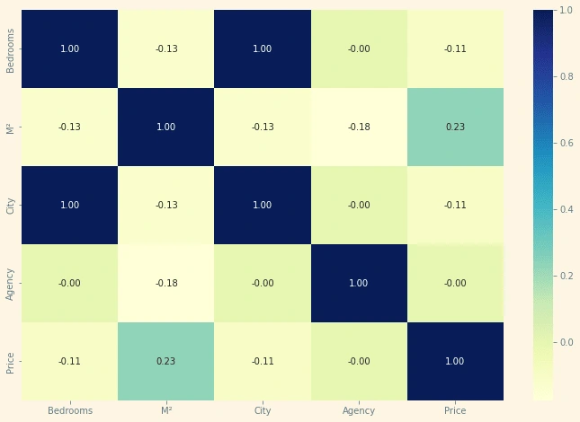
We can see that M², city and number of bedroom has a strong impact on the price
In [448]:
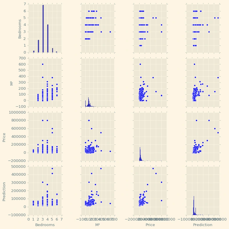
sns.pairplot(df)
Out[448]:
<seaborn.axisgrid.PairGrid at 0x7fcd742dbc90>
Machine Learning:
In [350]:
from sklearn.model_selection import train_test_splitimport xgboost as xgbfrom sklearn.metrics import mean_squared_errorfrom sklearn import metricsfrom sklearn.metrics import r2_score
In [410]:
X= df2.drop(columns=['Price'],axis=1)Y= df2['Price']
In [411]:
X_train, X_test, y_train, y_test = train_test_split(X, Y, test_size = 0.15, random_state = 100)
In [399]:
from sklearn.ensemble import GradientBoostingRegressorgbr = GradientBoostingRegressor()
In [414]:
gbr.fit(X_train,y_train)
Out[414]:
GradientBoostingRegressor()
In [415]:
score1 = gbr.score(X_train,y_train)score1
Out[415]:
0.4829150843528369
In [416]:
y_pred1 = gbr.predict(X_test)rscore1=r2_score(y_test, y_pred1)rscore1
Out[416]:
0.41718806361087724
In [431]:
df['Prediction']= gbr.predict(X)
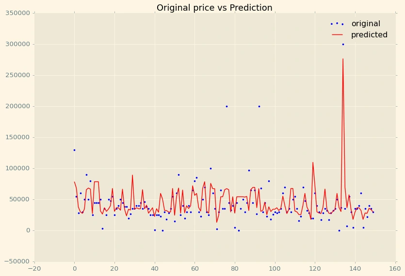
Price vs Prediction:
In [488]:
x_ax = range(len(df['Price'].head(150)))plt.figure(figsize=(12,8))plt.title('Original price vs Prediction')plt.scatter(x_ax, df['Price'].head(150), s=5, color="blue", label="original")plt.plot(x_ax, df['Prediction'].head(150), lw=1.3, color="red", label="predicted")plt.legend()plt.show()
Github link:
Like this project
Posted Mar 24, 2024
Data analysis Project