Predictive Modeling: Cars-For-Hire Ride Value Prediction 🚕

Overview 🔎

This is a use case I did for a mobility company to predict locations that yield the highest ride value based on time, latitude, and longitude values.

Check out the code here or click on the link below 🕵️‍♀️.

GitHub - Value Based Order Location Anticipation

GitHub - Value Based Order Location Anticipation





Medium - Regression Modeling: Taxi Rides Demand Prediction

Medium - Regression Modeling: Taxi Rides Demand Prediction



Problem & Solution 🤝

The availability of supply depends on the duration of time it takes for the drivers to reach the customers. The work explores the viability of algorithmic order location anticipation based on the data provided to guide the driver toward areas of the highest ride value.

What I did:

• Explored the viability of algorithmic order location anticipation based on the data provided to guide the driver toward areas of the highest ride value.
• Built a documented simple baseline model.
• Described how I would deploy such a model.
• Thought through and described the randomized experiment (AB-test) for live operations.

Problem statement: Based on the given dataset, can we predict locations that will yield the highest ride value, so that drivers can be guided to the locations before the time?

Goal: to use the dataset to predict ride values.

Metrics: A regression problem. Use mean squared error loss and R2 accuracy.

Application: predict ride values of each postcode location at every hour of the day, and return the top results.

Tech stacks used: scikit-learn, pandas, matplotlib, seaborn, geopy, folium, datetime, pickle, jupyter notebook.



Data 🗃

The source data is approximately 630,000 rows of synthetic ride demand data which resembles the real-life situation in the city of Tallinn. The columns include:

• the time of order
• the latitude and longitude of the start location
• the latitude and longitude of the destination
• the amount of money made on this ride



Process 🛣

Step 1: Data Loading

Data is loaded and checked if it contains null values. Then, the first 10,000 rows are extracted to be used for the rest of the code project to save computation time.

Observation: The data subset has no missing values. The column "ride_value" seems to have a large range of values.

Step 2: Data Cleaning

The column "start time" is processed into separate columns of date, time, hour, minute, and second. This is done to hopefully make the modeling process converge better.

Step 3: Feature Engineering

A few features are added to the dataset, which can be contextually helpful. They are day_of_week, is_weekend, start_postcode, and ride_distance.

• day_of_week: which day it is at the value of column "start_date". 1 = Monday, 7 = Sunday, and so on.
• is_weekend: whether the value of column "start_date" falls on a weekend. 0 = not a weekend, 1 = is a weekend.
• start_postcode: get the postcode of the pickup location based on values of columns "start_lat" and "start_lng".
• ride_distance: distance in kilometers between the pickup location and destination. End coordinates minus start coordinates.

Note: Postcodes might be useful when applied in reality. Drivers can check the top ride value areas based on postcodes. Maps can be visualized based on postcodes instead of pinpointing location coordinates. That's why I added this feature.

• Rows that have no postcode detected are removed.
• Columns "day_of_week" and "start_postcode" are label-encoded to hopefully yield better convergence in regression modeling.
• Different versions of preprocessed dataframes, as well as label encoders, are saved along the way.

Step 4: Machine Learning Modelling and Evaluation

Final features are selected for the use of ML modeling.

• The selected columns for Inputs are: start_lat, start_lng, start_postcode_encoded, start_time_hour, start_time_minute, start_time_second, end_lat, end_lng, day_of_week_encoded, is_weekend, and ride_distance.
• The selected column for Ground Truth is ride_value.

Train-test-split is performed with an 80% train set and a 20% test set. The validation set is not explicitly generated, as it will be done in cross-validation.

Three models are applied to the dataset in their default parameters for 5-fold cross-validation.

• They are linear regression, random forest regressor, and gradient boosting regressor.
• The model with the best score is further evaluated with the test set.
• Plots of y_test and y_pred are presented to see the comparison.



Results 📊

The best model is Linear Regression with a mean cross-validation score (MSE) of 0.154. Its test loss score is 0.007 and its test accuracy score is 0.996.



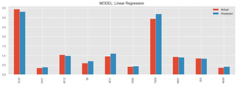
The first plot: a comparison between the actual and predicted ground truths of the first 10 ride values.



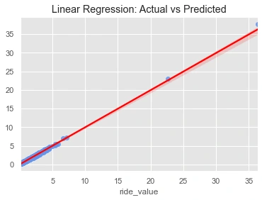
The second plot: the fit of the regression model on the actual and predicted ground truths of all ride values.



Answering the Problem Statement🎁

Statement: Based on the given dataset, can we predict locations that will yield the highest ride value, so that drivers can be guided to the locations before the time?

Answer: Based on the baseline model, we can predict ride value for each location, and the ride values can be ranked to return the top locations that will potentially yield the highest ride value. Drivers can then be informed and guided to these locations before the time.

Potential for further optimization:

• Data: consider including the weather dataset, DateTime, and address of local events and holidays and airline schedules. Use the full dataset instead of a subset.
• Models: consider optimizing models with hyperparameter optimization.
• Methodologies: consider implementing spatiotemporal forecasting models [1][2].
• [1] https://www.sciencedirect.com/science/article/abs/pii/S0968090X20305805
• [2] https://link.springer.com/article/10.1007/s42421-021-00041-4



Model Deployment🔌

Server

• Model training and optimization are carried out on the server side. Example: AWS EC2.
• New models can be automatically deployed in the server using the CI/CD pipeline.

Notebooks

• Jupyter Notebooks are used to do data analysis and modeling. Example: AWS Sagemaker.
• The trained model is optimized and saved in the database. Example: pickle file.

Database

• The model and dataset are hosted and archived on a chosen cloud storage. Example: AWS S3.

APIs

• On-demand prediction: create a REST API with a "predict" POST request. Example: Flask.
• It receives an input, preprocesses the data, uses the model to predict data, and returns a series of predicted ride values.
• Batch prediction: create an automated scheduler that batch predicts input data every day. Example: Apache Airflow.

Frontend applications: web and/or mobile

• Batch prediction scenario: the web or mobile backend receives a new batch of predictions every day. For every hour of the day, predict the ride value for every postcode. Use the backend to sort the ride value and return the top 3 ride value locations for every hour. Drivers can interact with a slider or a map to know which areas have the highest ride value of that day.
• On-demand prediction scenario: drivers input a postcode or location coordinate, as well as a chosen hour of the day. The Enter key sends input to the API and receives a ride value.



A/B Test Design for Live Operations ⚖️

User base

• Control group A: customer base using the existing app without the functionality of knowing higher ride value locations.
• Test group B: customer base using an updated app with the functionality of knowing higher ride value locations.

Metrics and hypotheses

• Metrics: hire-ride-ratio / driver idle time / customer wait time / cancel rate / hire completion rate.
• Hypothesis: Test group B will have a higher hire-ride ratio compared to control group A.
• Null hypothesis: There is no significant difference between the test and control groups.

A/B test design

• Select a dedicated sample size for Control group A and Test group B using random sampling.
• Deploy an updated app to a dedicated sample size as Test group B.
• Measure the hire-ride ratio for both groups for a set period of time.
• After data is collected, compare the hire-ride ratio for both groups. Get preliminary results, for example, Test group B has a higher hire-ride-ratio compared to Control group A.
• Check if the result is statistically significant. Use the ttest_ind() function of the Scipy library for T-test calculation.
• The ttest_ind() function returns two values: t-statistics and p-value.
• T-statistics quantifies the difference between the arithmetic means of the test and control groups.
• A higher t-statistic value means a larger difference between the average standard error between the two groups, which supports our hypothesis.
• P-value quantifies the probability of the null hypothesis being true.
• A p-value lower than 0.05 will make the null hypothesis invalid. It means that the test and control groups are statistically significant.
• Make a business decision based on the A/B test result.



👋Thanks for checking out my work. If this is similar or related to something you need to get done, I'd love to help you reach your goals. Feel free to reach out, I'm curious to know more about your use case! 🤩