Comprehensive Stock Analysis and Prediction Using LSTM: A Case …

In the fast-paced world of stock trading, the ability to analyze and predict stock price movements is crucial for making informed investment decisions. This project leverages historical stock data from the National Stock Exchange of India (NSE) to identify undervalued stocks and predict future price trends using advanced machine learning techniques.

The project begins with data acquisition, where I used the Yahoo Finance API to gather daily stock price data for major Indian companies, including Reliance Industries (RELIANCE.NS), Tata Consultancy Services (TCS.NS), Infosys (INFY.NS), HDFC Bank (HDFCBANK.NS), ICICI Bank (ICICIBANK.NS), and State Bank of India (SBIN.NS).I have used 5 companies for showcase it can be easily used for more. The dataset spans the past year, providing a robust foundation for both analysis and forecasting.

1. Undervaluation Screening: We implement a screening process to identify undervalued stocks based on significant downward movements from their 7-day average closing prices. This involves calculating daily price movements and ranking stocks to highlight those with the greatest deviation from their recent average.

2. Data Enrichment: Additional market data, such as market movement, industry movement, and index movement, is integrated into the dataset to provide a more comprehensive view of stock performance relative to broader market trends.

3. Data Filtering: The project applies various filters to refine the list of undervalued stocks. These filters include fundamental strength and popularity criteria, as well as market size rankings to ensure the selection of robust investment opportunities.

4. Visualization: Using Plotly, we create visual representations of the undervalued stocks, including bar charts to display movement percentages and line charts to visualize historical price trends for specific stocks.

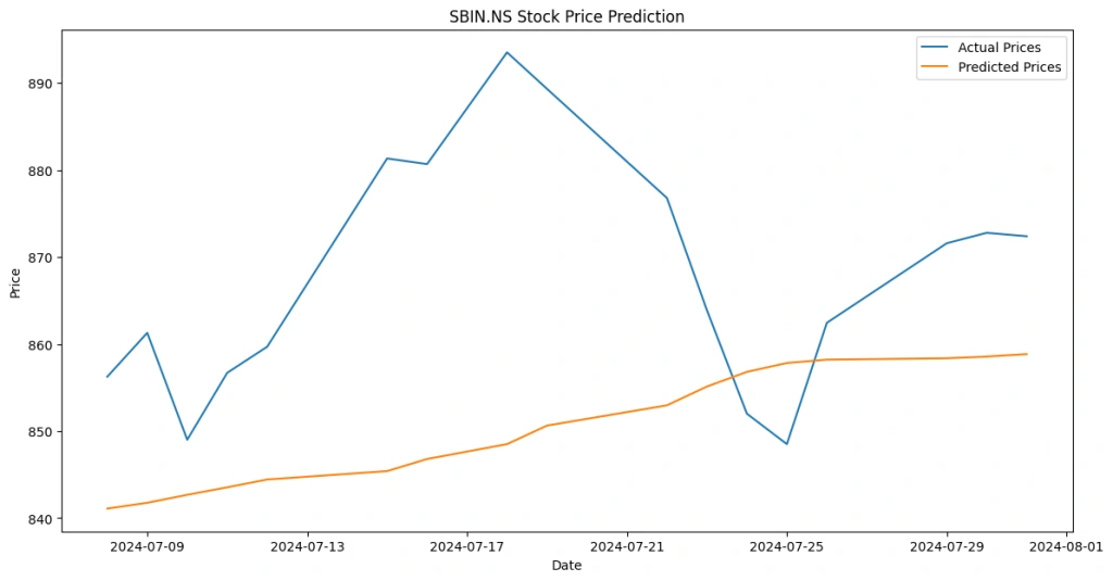
5. Prediction Modeling: To forecast future stock prices, we employ Long Short-Term Memory (LSTM) networks, a type of recurrent neural network (RNN) well-suited for time series prediction. This involves training an LSTM model on historical price data and evaluating its performance with a focus on prediction accuracy.

This project not only provides a tool for identifying and analyzing undervalued stocks but also offers insights into future price movements, aiding investors in making data-driven decisions. Through detailed data processing, visualization, and predictive modeling, the project demonstrates a practical approach to stock market analysis and forecasting.

import yfinance as yf import pandas as pd import numpy as np from datetime import datetime, timedelta

end_date = datetime.today() start_date = end_date – timedelta(days=365) # For a year of data

tickers = [ ‘RELIANCE.NS’, ‘TCS.NS’, ‘INFY.NS’, ‘HDFCBANK.NS’, ‘ICICIBANK.NS’,’SBIN.NS’

]

def fetch_data(tickers, start_date, end_date): data = {} for ticker in tickers: try: df = yf.download(ticker, start=start_date, end=end_date, interval=’1d’) df[‘Ticker’] = ticker data[ticker] = df except Exception as e: print(f”Error fetching data for {ticker}: {e}”) return data

def calculate_movement(df): df[‘7day_avg’] = df[‘Close’].rolling(window=7).mean() df[‘Movement’] = (df[‘Close’] – df[‘7day_avg’]) / df[‘7day_avg’] * 100 return df

def screen_undervalued_stocks(data): undervalued = [] for ticker, df in data.items(): df = calculate_movement(df) latest_movement = df.iloc[-1][‘Movement’] undervalued.append((ticker, latest_movement)) undervalued.sort(key=lambda x: x[1], reverse=True) return undervalued

def get_stock_data(): data = fetch_data(tickers, start_date, end_date) undervalued_stocks = screen_undervalued_stocks(data) return undervalued_stocks

undervalued_stocks = get_stock_data()

df = pd.DataFrame(undervalued_stocks, columns=[‘Ticker’, ‘Movement’]) df = df.sort_values(by=’Movement’, ascending=False)

df.to_csv(‘undervalued_stocks.csv’, index=False)

print(df)

Ticker Movement

0 ICICIBANK.NS 1.822643

1 RELIANCE.NS 0.754712

2 SBIN.NS 0.125430

3 TCS.NS 0.016964

4 INFY.NS 0.003452

5 HDFCBANK.NS -0.140018

def fetch_market_data(): return { ‘Market_Movement’: 1.5, ‘Industry_Movement’: 2.0, ‘Index_Movement’: 0.5 }

def integrate_additional_fields(df): market_data = fetch_market_data() df[‘Market_Movement’] = market_data[‘Market_Movement’] df[‘Industry_Movement’] = market_data[‘Industry_Movement’] df[‘Index_Movement’] = market_data[‘Index_Movement’] return df

df = integrate_additional_fields(df) df.to_csv(‘undervalued_stocks_with_movements.csv’, index=False)

def apply_filters(df):

filtered_df = df[df[‘Movement’] > -5] return filtered_df

df_filtered = apply_filters(df) df_filtered.to_csv(‘filtered_undervalued_stocks.csv’, index=False)

import plotly.express as px import pandas as pd

def plot_undervalued_stocks_plotly(df): fig = px.bar(df, x=’Ticker’, y=’Movement’, title=’Undervalued Stocks Based on Movement’, labels={‘Movement’: ‘Movement (%)’, ‘Ticker’: ‘Stock Ticker’}, color=’Movement’, color_continuous_scale=px.colors.sequential.Inferno) fig.update_layout(xaxis_title=’Stock Ticker’, yaxis_title=’Movement (%)’, xaxis_tickangle=-45) fig.show()

df = pd.read_csv(‘undervalued_stocks.csv’) plot_undervalued_stocks_plotly(df)

After Undervaluation Screening I have used SBIN for simplicity same can be used for others also.

import yfinance as yf import pandas as pd import plotly.express as px

def fetch_data_multiple_days(ticker, start_date, end_date, interval=’1d’):

stock = yf.Ticker(ticker)

data = stock.history(start=start_date, end=end_date, interval=interval)

data = data.reset_index()

return data

def plot_stock_data(ticker, start_date, end_date, interval=’1d’): df = fetch_data_multiple_days(ticker, start_date, end_date, interval)

if df.empty: print(f”No data available for ticker {ticker} between {start_date} and {end_date}.”) return

fig = px.line(df, x=’Date’, y=’Close’, title=f’Stock Prices for {ticker} from {start_date} to {end_date}’, labels={‘Close’: ‘Price ($)’, ‘Date’: ‘Date’})

fig.update_layout(xaxis_title=’Date’, yaxis_title=’Price ($)’) fig.show()

plot_stock_data(‘SBIN.NS’, ‘2023-08-10’, ‘2024-08-10′, interval=’1d’)

from sklearn.preprocessing import MinMaxScaler from sklearn.model_selection import train_test_split import tensorflow as tf from tensorflow.keras.models import Sequential from tensorflow.keras.layers import LSTM, Dense import matplotlib.pyplot as plt

def fetch_data(ticker, start_date, end_date): stock = yf.Ticker(ticker) data = stock.history(start=start_date, end=end_date) return data

def prepare_data(df, feature_col=’Close’, look_back=60): data = df[[feature_col]].values scaler = MinMaxScaler(feature_range=(0, 1)) scaled_data = scaler.fit_transform(data)

X, y = [], [] for i in range(len(scaled_data) – look_back): X.append(scaled_data[i:i+look_back]) y.append(scaled_data[i+look_back])

X, y = np.array(X), np.array(y) return X, y, scaler

def build_lstm_model(input_shape): model = Sequential() model.add(LSTM(50, return_sequences=True, input_shape=input_shape)) model.add(LSTM(50)) model.add(Dense(1)) model.compile(optimizer=’adam’, loss=’mean_squared_error’) return model

ticker = ‘SBIN.NS’ start_date = ‘2024-01-01’

data = fetch_data(ticker, start_date, end_date) X, y, scaler = prepare_data(data)

X_train, X_test, y_train, y_test = train_test_split(X, y, test_size=0.2, shuffle=False)

model = build_lstm_model(input_shape=(X_train.shape[1], X_train.shape[2])) history = model.fit(X_train, y_train, epochs=20, batch_size=32, validation_split=0.1)

predictions = model.predict(X_test) predictions = scaler.inverse_transform(predictions) y_test = scaler.inverse_transform(y_test)

plt.figure(figsize=(14, 7)) plt.plot(data.index[-len(y_test):], y_test, label=’Actual Prices’) plt.plot(data.index[-len(y_test):], predictions, label=’Predicted Prices’) plt.xlabel(‘Date’) plt.ylabel(‘Price’) plt.title(f'{ticker} Stock Price Prediction’) plt.legend() plt.show()