Taxi Service Dynamic Pricing Strategy using Machine Learning

Smruti Pote

Completed work

Data Scientist

LangChain

MySQL

pandas

Artificial Intelligence

Taxi Service Dynamic Pricing Strategy using Machine Learning

Smruti Pote

6 min read

Apr 6, 2025

Dynamic Pricing is a data science technique used to modify product or service prices in real time based on multiple factors. Businesses leverage it to maximize revenue by setting adaptable prices that reflect market demand, customer behavior, demographics, and competitor pricing. If you’re interested in creating a data-driven Dynamic Pricing Strategy, this article will guide you through the process using Python.

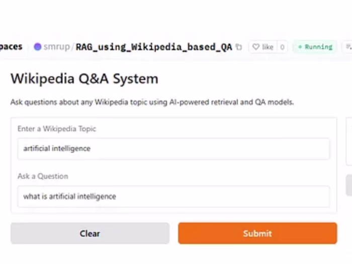
Try is yourself :https://huggingface.co/spaces/smrup/Taxi_Dynamic_Pricing_Strategy

What is Dynamic Pricing?

Dynamic Pricing is a data science approach that involves modifying the price of products or services in real time, based on various influencing factors. Businesses use this strategy to enhance revenue and profitability by setting prices that adapt to market demand, customer behavior, and competitor activity.

By leveraging data-driven insights and advanced algorithms, companies can continuously adjust prices to achieve optimal outcomes.

Take, for instance, a ride-sharing service in a city. Traditionally, such companies use fixed pricing per kilometer, which doesn’t reflect changes in real-time demand or supply.

With a dynamic pricing model, the company can utilize data science to analyze elements like past ride data, current demand levels, traffic conditions, and local events. Machine Learning algorithms help interpret this data and enable real-time price adjustments. During peak hours or large events, prices may rise to encourage more drivers to operate, balancing supply and demand. In contrast, prices can be reduced during off-peak times to attract more rides.

Dynamic Pricing Strategy: Overview

So, in a dynamic pricing strategy, the aim is to maximize revenue and profitability by pricing items at the right level that balances supply and demand dynamics. It allows businesses to adjust prices dynamically based on factors like time of day, day of the week, customer segments, inventory levels, seasonal fluctuations, competitor pricing, and market conditions.

To implement a data-driven dynamic pricing strategy, businesses typically require data that can provide insights into customer behaviour, market trends, and other influencing factors. So to create a dynamic pricing strategy, we need to have a dataset based on:

historical sales data

customer purchase patterns

market demand forecasts

cost data

customer segmentation data,

Real-time market data.

I found an ideal dataset to create a Dynamic Pricing Strategy based on the example we discussed above. You can download the data from here.

Dynamic Pricing Strategy using Python

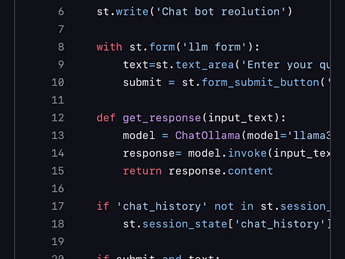
Let’s start the task of building a dynamic pricing strategy by importing the necessary Python libraries and the dataset:

df= pd.read_csv('dynamic_pricing.csv')df.head()

Exploratory Data Analysis

Let’s have a look at the descriptive statistics of the data: (data.describe())

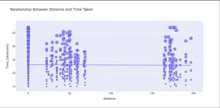
Now let’s have a look at the relationship between expected ride duration and the historical cost of the ride:

fig = px.scatter(data, x='Expected_Ride_Duration',                  y='Historical_Cost_of_Ride',                 title='Expected Ride Duration vs. Historical Cost of Ride',                  trendline='ols')fig.show()

Now let’s have a look at the distribution of the historical cost of rides based on the vehicle type:

Now let’s have a look at the correlation matrix:

corr_matrix = df[['Number_of_Riders', 'Number_of_Drivers','Number_of_Past_Rides', 'Average_Ratings',       'Expected_Ride_Duration',       'Historical_Cost_of_Ride']].corr()fig = go.Figure(data=go.Heatmap(z=corr_matrix.values,                                 x=corr_matrix.columns,                                 y=corr_matrix.columns,                                colorscale='Viridis'))fig.update_layout(title='Correlation Matrix')fig.show()

Implementing a Dynamic Pricing Strategy

According to the company’s data, their current pricing model relies solely on the estimated ride duration to determine ride costs. In this project, we’ll implement a dynamic pricing strategy that adjusts ride prices based on fluctuations in demand and supply. The goal is to raise prices during periods of high demand or low driver availability, and lower them when demand is low or supply is abundant.

import numpy as np# Calculate demand_multiplier based on percentile for high and low demandhigh_demand_percentile = 75low_demand_percentile = 25data['demand_multiplier'] = np.where(data['Number_of_Riders'] > np.percentile(data['Number_of_Riders'], high_demand_percentile),                                     data['Number_of_Riders'] / np.percentile(data['Number_of_Riders'], high_demand_percentile),                                     data['Number_of_Riders'] / np.percentile(data['Number_of_Riders'], low_demand_percentile))# Calculate supply_multiplier based on percentile for high and low supplyhigh_supply_percentile = 75low_supply_percentile = 25data['supply_multiplier'] = np.where(data['Number_of_Drivers'] > np.percentile(data['Number_of_Drivers'], low_supply_percentile),                                     np.percentile(data['Number_of_Drivers'], high_supply_percentile) / data['Number_of_Drivers'],                                     np.percentile(data['Number_of_Drivers'], low_supply_percentile) / data['Number_of_Drivers'])# Define price adjustment factors for high and low demand/supplydemand_threshold_high = 1.2  # Higher demand thresholddemand_threshold_low = 0.8  # Lower demand thresholdsupply_threshold_high = 0.8  # Higher supply thresholdsupply_threshold_low = 1.2  # Lower supply threshold# Calculate adjusted_ride_cost for dynamic pricingdata['adjusted_ride_cost'] = data['Historical_Cost_of_Ride'] * (    np.maximum(data['demand_multiplier'], demand_threshold_low) *    np.maximum(data['supply_multiplier'], supply_threshold_high))

In the above code, we begin by calculating the demand multiplier. This is done by comparing the current number of riders to predefined percentile thresholds for high and low demand. If rider count exceeds the high-demand percentile, the multiplier is calculated as the ratio of riders to that percentile. Conversely, if it falls below the low-demand threshold, we use the ratio of riders to the low-demand percentile.

We then compute the supply multiplier by assessing the number of available drivers against the high and low supply percentiles. If driver count is above the low-supply percentile, the multiplier is set as the high-supply percentile divided by the number of drivers. If driver availability is below the low-supply percentile, we use the low-supply percentile divided by the driver count.

Lastly, we determine the dynamically adjusted ride cost by multiplying the original ride cost by the greater of the demand multiplier or a minimum threshold (demand_threshold_low), and also by the greater of the supply multiplier or a maximum threshold (supply_threshold_high). These thresholds help regulate extreme fluctuations, ensuring price changes stay within reasonable bounds.

Now, let’s move on to calculating the profit percentage achieved through this dynamic pricing approach.

# Calculate the profit percentage for each ridedata['profit_percentage'] = ((data['adjusted_ride_cost'] - data['Historical_Cost_of_Ride']) / data['Historical_Cost_of_Ride']) * 100# Identify profitable rides where profit percentage is positiveprofitable_rides = data[data['profit_percentage'] > 0]# Identify loss rides where profit percentage is negativeloss_rides = data[data['profit_percentage'] < 0]import plotly.graph_objects as go# Calculate the count of profitable and loss ridesprofitable_count = len(profitable_rides)loss_count = len(loss_rides)# Create a donut chart to show the distribution of profitable and loss rideslabels = ['Profitable Rides', 'Loss Rides']values = [profitable_count, loss_count]fig = go.Figure(data=[go.Pie(labels=labels, values=values, hole=0.4)])fig.update_layout(title='Profitability of Rides (Dynamic Pricing vs. Historical Pricing)')fig.show()

Training a Predictive Model

Now, as we have implemented a dynamic pricing strategy, let’s train a Machine Learning model. Before training the model, let’s preprocess the data:

import pandas as pdimport numpy as npfrom sklearn.preprocessing import StandardScalerdef data_preprocessing_pipeline(data):    #Identify numeric and categorical features    numeric_features = data.select_dtypes(include=['float', 'int']).columns    categorical_features = data.select_dtypes(include=['object']).columns    #Handle missing values in numeric features    data[numeric_features] = data[numeric_features].fillna(data[numeric_features].mean())    #Detect and handle outliers in numeric features using IQR    for feature in numeric_features:        Q1 = data[feature].quantile(0.25)        Q3 = data[feature].quantile(0.75)        IQR = Q3 - Q1        lower_bound = Q1 - (1.5 * IQR)        upper_bound = Q3 + (1.5 * IQR)        data[feature] = np.where((data[feature] < lower_bound) | (data[feature] > upper_bound),                                 data[feature].mean(), data[feature])    #Handle missing values in categorical features    data[categorical_features] = data[categorical_features].fillna(data[categorical_features].mode().iloc[0])    return data

Now let’s split the data and train a Machine Learning model to predict the cost of a ride:

#splitting datafrom sklearn.model_selection import train_test_splitx = np.array(data[["Number_of_Riders", "Number_of_Drivers", "Vehicle_Type", "Expected_Ride_Duration"]])y = np.array(data[["adjusted_ride_cost"]])x_train, x_test, y_train, y_test = train_test_split(x,                                                    y,                                                    test_size=0.2,                                                    random_state=42)# Reshape y to 1D arrayy_train = y_train.ravel()y_test = y_test.ravel()# Training a random forest regression modelfrom sklearn.ensemble import RandomForestRegressormodel = RandomForestRegressor()model.fit(x_train, y_train)

def get_vehicle_type_numeric(vehicle_type):    vehicle_type_mapping = {        "Premium": 1,        "Economy": 0    }    vehicle_type_numeric = vehicle_type_mapping.get(vehicle_type)    return vehicle_type_numeric  # Predicting using user input valuesdef predict_price(number_of_riders, number_of_drivers, vehicle_type, Expected_Ride_Duration):    vehicle_type_numeric = get_vehicle_type_numeric(vehicle_type)    if vehicle_type_numeric is None:        raise ValueError("Invalid vehicle type")        input_data = np.array([[number_of_riders, number_of_drivers, vehicle_type_numeric, Expected_Ride_Duration]])    predicted_price = model.predict(input_data)    return predicted_price# Example prediction using user input valuesuser_number_of_riders = 50user_number_of_drivers = 25user_vehicle_type = "Economy"Expected_Ride_Duration = 30predicted_price = predict_price(user_number_of_riders, user_number_of_drivers, user_vehicle_type, Expected_Ride_Duration)print("Predicted price:", predicted_price)

Check out the complete code here: https://github.com/smrutipote/Taxi-Cab-Dynamic-Pricing-Strategy

Also don’t forget to try this strategy which is deployed live : https://huggingface.co/spaces/smrup/Taxi_Dynamic_Pricing_Strategy

Like this project

Completed work

Posted Apr 18, 2025

Developed a dynamic pricing strategy for a taxi service using Python and machine learning.

Likes

Views