Food Delivery Time Prediction using Machine Learning
Smruti Pote

Food Delivery Time Prediction using Machine Learning
·
7 min read
·
Apr 5, 2025
🛵 Food Delivery Time Prediction with Machine Learning
Companies like Zomato and Swiggy need to give users an accurate estimate of how long it will take to deliver their food. This helps: Build trust with customers 🧑🍳Improve user experience 📱Optimize delivery operations 🚴But how do they do it?
They use Machine Learning (ML)! 🧠
ML models are trained to predict delivery time based on past data — like how long it took delivery partners to travel similar distances under similar conditions.
🧪 What This Article Covers
If you’re curious about how this works under the hood, you’re in the right place. This article covers how to build a food delivery time prediction system using: Historical delivery data (e.g., distance, delivery time, traffic). Python and popular libraries like
scikit-learn or GradientBoostA real Machine Learning model that predicts time taken to deliver an order which includes Data collection and preprocessing, Feature engineering (e.g., extracting time of day, day of week), Model training and evaluation, Making predictions on new delivery orders.So, for this task, we need a dataset containing data about the time taken by delivery partners to deliver food from the restaurant to the delivery location. I found an ideal dataset with all the features for this task. You can download the dataset from here.
Food Delivery Time Prediction using Python
I will start the task of food delivery time prediction by importing the necessary Python libraries and the dataset:
Let’s have a look at the column insights before moving forward:
Now let’s have a look at whether this dataset contains any null values or not:
There are no missing values in the dataset, so we’re good to go!
Calculating the Distance Between Two Coordinates
The dataset doesn’t directly provide the distance between the restaurant and the delivery address. Instead, it gives us the latitude and longitude for both points. To estimate the distance between them, we can apply the Haversine formula, which calculates the great-circle distance between two points on a sphere based on their geographic coordinates.
Here’s how you can compute the distance between the restaurant and the delivery location using the Haversine formula:
This sets the radius of the Earth in kilometers. It’s a constant used in the Haversine formula to convert angular distance (in radians) to actual distance (in km).Since most trigonometric functions in NumPy (like
sin, cos) expect radians, this helper function converts degrees to radians. Formula: radians = degrees × π / 180d_lat and d_lon are the differences in latitude and longitude, converted to radians. Initializes a new column called 'distance' in the DataFrame with NaN values. Loops through each row in the DataFrame. For each row, it: Retrieves the latitude/longitude of the restaurant and delivery location. Calculates the distance using distcalculate(). Stores the result in the 'distance' column.We have now calculated the distance between the restaurant and the delivery location. We have also added a new feature in the dataset as distance. Let’s look at the dataset again:
Data Exploration
Now let’s explore the data to find relationships between the features. I’ll start by looking at the relationship between the distance and time taken to deliver the food:
There appears to be a steady pattern between the delivery time and the distance covered. This suggests that most delivery partners complete deliveries in about 25 to 30 minutes, regardless of how far they have to travel.
Next, let’s explore how delivery time varies based on the age of the delivery partner.
here is a linear relationship between the time taken to deliver the food and the age of the delivery partner. It means young delivery partners take less time to deliver the food compared to the elder partners.
Now let’s have a look at the relationship between the time taken to deliver the food and the ratings of the delivery partner:
There is an inverse linear relationship between the time taken to deliver the food and the ratings of the delivery partner. It means delivery partners with higher ratings take less time to deliver the food compared to partners with low ratings.
Now let’s have a look if the type of food ordered by the customer and the type of vehicle used by the delivery partner affects the delivery time or not:
There isn’t a significant variation in delivery times based on the type of vehicle used or the kind of food being delivered.
Based on our analysis, the key factors that have the most impact on food delivery time are: The age of the delivery partner, The ratings of the delivery partner. The distance between the restaurant and the delivery location.
In the following section, we’ll walk through the process of training a Machine Learning model to predict food delivery times.
Food Delivery Time Prediction Model
This code demonstrates a complete machine learning workflow for predicting food delivery time using three different regression models: Linear Regression, Random Forest Regressor, and Gradient Boosting Regressor.
It starts by selecting relevant features — delivery partner’s age, their rating, and the distance between the restaurant and delivery location — as the input variables (X), and the delivery time in minutes as the target variable (y). The dataset is then split into training and testing sets using an 80–20 ratio. Each model is trained on the training data and used to make predictions on the test set.
The performance of the models is evaluated using metrics such as Mean Absolute Error (MAE), Root Mean Squared Error (RMSE), and R² score, which indicate the accuracy of the predictions. Finally, the results from all three models are compared and summarized in a DataFrame, allowing us to easily assess which model performs best for predicting food delivery times.
Summary
To accurately predict food delivery time in real-time, it’s essential to calculate the distance between the location where the food is prepared and the customer’s address. Once this distance is determined, the next step is to analyze historical data to identify patterns in how long delivery partners have typically taken to cover similar distances.
This helps build a reliable prediction model. I hope you found this article on predicting food delivery time using Machine Learning in Python insightful and useful.
Check out the code and repository on github :https://github.com/smrutipote/Food-Delivery-Time-using-Machine-Learning
Also check out this project live on huggingface : https://huggingface.co/spaces/smrup/Food-Delivery-Time-Prediction-using-Machine-Learning
Like this project
Posted Apr 18, 2025
Built a ML model to predict food delivery times using Python and historical data.
Likes
0
Views
4