Research Data Analysis and Visualization
Hadi Rajabbeigi
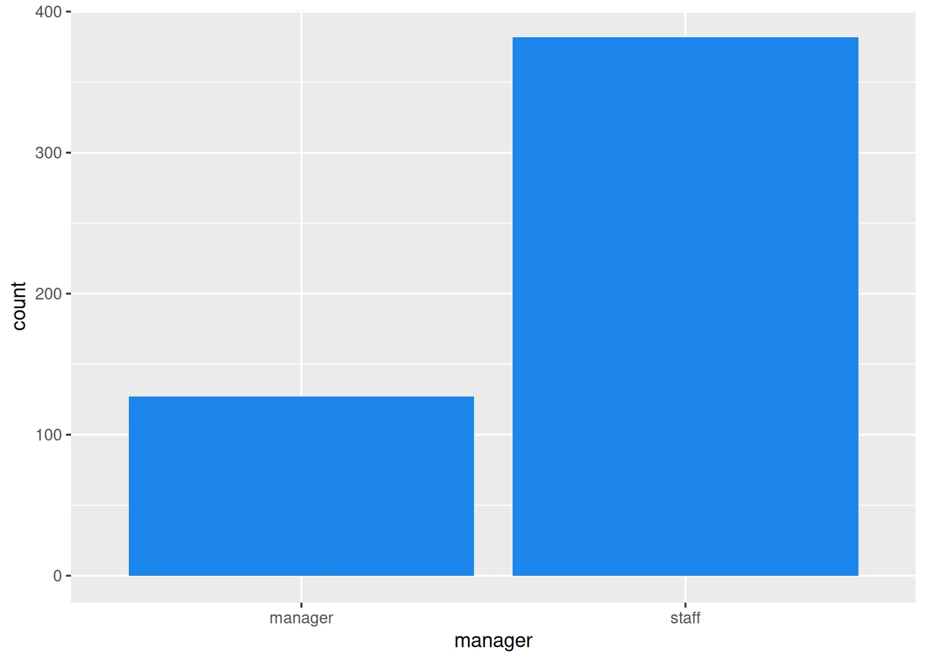
Table of contents
Author
Importing Data
Data was imported from spss file james.sav which was provided by Dr. Dellaneve:
Selecting Required Data
Some of the columns was omitted from dataset and a report from current variables and their frequency created as a PDF file and the data saved as a new data file:
Creating Categorical Variables
In this step, the categorical variables such as gender, race, education, etc. was created from related questions:
Computing Continuous Variables
In this step, continuous (dependent) variables was calculated (took mean):
Categorical Visualization
Management Status Bar Chart:
Gender Bar Charts:
Generation
Race
States
Education
Employment Status
Industries
Spearman Correlations
In this step the Spearman correlations between questions of the study is created:
Anxiety Items
Avoidance Items
Interpersonal Deviance Items
ACE Items
Self-Attachment Items
All Items (Q08 to Q112)
Scatter Plots
Anxiety vs. Avoidance
Interpersonal Deviance vs. Anxiety
Interpersonal Deviance vs. Avodiance
Organizational Deviance vs. Avoidance
OrgDev vs. Anxiety
Test of Normality
Employee Engagement
Self-Attachment
Phubbing
Remote Teams
Focus
Anxiety
Avoidance
Interpersonal Deviance
Organizational Deviance
ACE
Kruskal Wallis Test
Since our continuous variables are not normally distributed, we used non-parametric test of Kruskal Wallis to find how the variables diverse among demographics:
Employee Engagement Vs. Demographics
As we see in the following results there is not any significant difference regarding employee engagement among demographics:
Self-Attachment Vs. Demographics
As the following results show, the self-attachment difference is significant for education and generation at p = 0.05
Phubbing
The results below show that phubbing has a significant difference in generation.
Remote Teams
Results indicate a significant difference for Remote Teams regarding generation
Focus
Results indicate focus has a significant difference regarding generation
Anxiety
Anxiety shows a significant difference in generation and gender
Avoidance
Interpersonal Deviance
Organizational Deviance
ACE
Post-Hocs
Interpersonal Deviance vs. Race
Interpersonal Deviance vs. Generation
Organizational Deviance vs Generation
ACE vs. Education
Avoidance vs. Generation
Anxiety vs. Generation
Interpersonal Deviance vs. Gender
Wilcoxon Test
Since Gender has two categories in our study (male and female) we used Wilcoxon test to find out about the difference among groups:
Employee Engagement vs. Gender
Self-Attachment vs. Gender
Phubbing vs. Gender
Remote vs. Gender
Focus vs. Gender
Anxiety vs. Gender
Avoidance vs. Gender
Interpersonal Deviance vs. Gender
Organizational Deviance vs. Gender
ACE vs. Gender
Means Across Demographics
We took mean for variables with a significant difference to see how different categories behave
Interpersonel Deviance vs. Race
Interpersonal Deviance vs. Generation
Interpersonal Deviance vs. Gender
Organizational Deviance vs. Generation
Organizational Deviance vs. Gender
Self-Attachement vs. Education
Phubbing vs. Generation
Remote vs. Generation
Focus vs. Generation
Anxiety vs. Generation
Anxiety vs. Gender
Avoidance vs. Generation
ACE vs. Education
Like this project
Posted May 25, 2025
Data analysis and visualization for Dr. Dellaneve's research.