·

Published in

·

9 min read

·

Jul 6, 2020

--

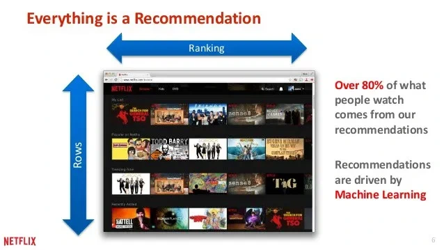
A recommender system, or a recommendation system (sometimes replacing ‘system’ with a synonym such as platform or engine), is a subclass of information filtering system that seeks to predict the “rating” or “preference” a user would give to an item. They are primarily used in commercial applications.

Recommender systems are utilized in a variety of areas and are most commonly recognized as playlist generators for video and music services like Netflix, YouTube and Spotify, product recommenders for services such as Amazon, or content recommenders for social media platforms such as Facebook and Twitter. These systems can operate using a single input, like music, or multiple inputs within and across platforms like news, books, and search queries. There are also popular recommender systems for specific topics like restaurants and online dating. Recommender systems have also been developed to explore research articles and experts, collaborators, and financial services.

In a very general way, recommender systems are algorithms aimed at suggesting relevant items to users (items being movies to watch, text to read, products to buy or anything else depending on industries).

Here we are going to overview some major paradigms of recommender systems : popularity,content based & collaborative filtering. The following section will be dedicated to all the above mentioned algorithms and how they work.

tdmb_5000_movies dataset

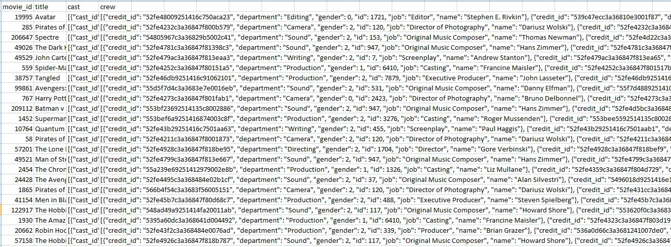
tdmb_5000_credits dataset

Now we merge the above datasets to proceed further:

As the name suggests Popularity based recommendation system works with the trend. It basically uses the items which are in trend right now. For example, if any product which is usually bought by every new user then there are chances that it may suggest that item to the user who just signed up.

Weighted Rating(WR)=[vR/(v+m)]+[mC/(v+m)] where, v is the number of votes for the movie; m is the minimum votes required to be listed in the chart; R is the average rating of the movie; and C is the mean vote across the whole report. Now we find the values of v,m,R,C.

(481, 23)

Here we used 90th percentile as our cutoff. In other words, for a movie to feature in the charts, it must have more votes than at least 90% of the movies in the list.

We see that there are 481 movies which qualify to be in this list. Now, we need to calculate our metric for each qualified movie. To do this, we will define a function, weighted_rating() and define a new feature score, of which we’ll calculate the value by applying this function to our DataFrame of qualified movies:

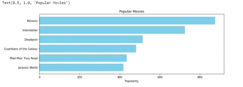
Now we visualize the top 6 movies according to popularity based recommender system.

Conclusion: The Popularity based recommender provide a general chart of recommended movies to all the users. They are not sensitive to the interests and tastes of a particular user.

In this recommender system the content of the movie (overview, cast, crew, keyword, tagline etc) is used to find its similarity with other movies. Then the movies that are most likely to be similar are recommended.

Plot description based Recommender: Here we will compute pairwise similarity scores for all movies based on their plot descriptions and recommend movies based on that similarity score. The plot description is given in the “overview” feature of our dataset.

(4803, 20978)

We see that 20978 different words were used to describe the 4803 movies in our dataset.

With this matrix, we compute a similarity score. We will be using the cosine similarity to calculate a numeric quantity that denotes the similarity between two movies. We use the cosine similarity score since it is independent of magnitude and is relatively easy and fast to calculate. Mathematically, it is defined as follows:

Since we have used the TF-IDF vectorizer, calculating the dot product will directly give us the cosine similarity score. Therefore, we will use sklearn’s linear_kernel() instead of cosine_similarities() since it is faster.

Now we need a mechanism to identify the index of a movie in our metadata DataFrame, given its title.

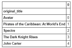
Now we need to to follow the steps for defining our recommendation function: *Getting the index of the movie given its title. *Getting the list of cosine similarity scores for that particular movie with all movies. *Converting it into a list of tuples where the first element is its position and the second is the similarity score. *Sorting the aforementioned list of tuples based on the similarity scores; that is, the second element. *Getting the top 10 elements of this list. Ignoring the first element as it refers to self (the movie most similar to a particular movie is the movie itself). *Returning the titles corresponding to the indices of the top elements.

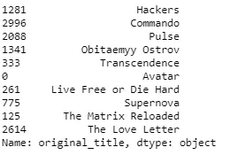
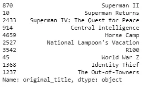
Conclusion: While our system has done a decent job of finding movies with similar plot descriptions, the quality of recommendations is not that great.

We are going to build a recommender based on the following: the 3 top actors, the director, related genres and the movie plot keywords. From the cast, crew and keywords features, we need to extract the three most important actors, the director and the keywords associated with that movie. Right now, our data is present in the form of “stringified” lists , we need to convert it into a safe and usable structure.

Our next step would be to convert the names and keyword instances into lowercase and strip all the spaces between them. This is done so that our vectorizer doesn’t count the Johnny of “Johnny Depp” and “Johnny Galecki” as the same.

Now we create our “metadata soup”, which is a string that contains all the metadata that we want to feed to our vectorizer (namely actors, director and keywords).

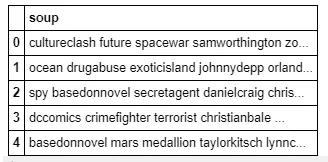
The next steps are the same as what we did with our plot description based recommender. One important difference is that we use the CountVectorizer() instead of TF-IDF. This is because we do not want to down-weight the presence of an actor/director if he or she has acted or directed in relatively more movies. It doesn’t make much intuitive sense.

Again we need to to follow the steps mentioned earlier for defining our recommendation function.

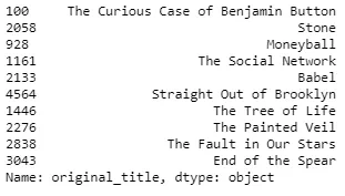
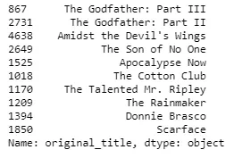
Conclusion: We see that our recommender has been successful in capturing more information due to more metadata and has given us (arguably) better recommendations. It is more likely that Marvels or DC comics fans will like the movies of the same production house. Therefore, to our features above we can add production_company . We can also increase the weight of the director , by adding the feature multiple times in the soup.

Our content based engine suffers from some severe limitations. It is only capable of suggesting movies which are close to a certain movie. That is, it is not capable of capturing tastes and providing recommendations across genres.

Also, the engine that we built is not really personal in that it doesn’t capture the personal tastes and biases of a user. Anyone querying our engine for recommendations based on a movie will receive the same recommendations for that movie, regardless of who she/he is.

Therefore, in this section, we will use a technique called Collaborative Filtering to make recommendations to Movie Watchers. It is basically of two types:-

User based filtering- These systems recommend products to a user that similar users have liked. For measuring the similarity between two users we can either use pearson correlation or cosine similarity.

Item Based Collaborative Filtering -Instead of measuring the similarity between users, the item-based CF recommends items based on their similarity with the items that the target user rated. Likewise, the similarity can be computed with Pearson Correlation or Cosine Similarity.

One way to handle the scalability and sparsity issue created by CF is to leverage a latent factor model to capture the similarity between users and items. Essentially, we want to turn the recommendation problem into an optimization problem. We can view it as how good we are in predicting the rating for items given a user. One common metric is Root Mean Square Error (RMSE). The lower the RMSE, the better the performance.

Now talking about latent factor you might be wondering what is it ?It is a broad idea which describes a property or concept that a user or an item have. For instance, for music, latent factor can refer to the genre that the music belongs to. SVD decreases the dimension of the utility matrix by extracting its latent factors. Essentially, we map each user and each item into a latent space with dimension r. Therefore, it helps us better understand the relationship between users and items as they become directly comparable.

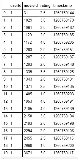
Now enough said , let’s see how to implement this. Since the dataset we used before did not have userId(which is necessary for collaborative filtering) let’s load another dataset. We’ll be using the Surprise library to implement SVD. So our first step is to install the Surprise library by using the command !pip install surprise .

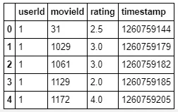
Note that in this dataset movies are rated on a scale of 5 unlike the earlier one.

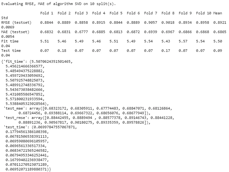
<surprise.prediction_algorithms.matrix_factorization.SVD at 0x7f372e7c2c88>

Prediction(uid=1, iid=302, r_ui=3, est=2.935174843805315, details={'was_impossible': False})

Conclusion: For movie with ID 302, we get an estimated prediction of 2.935. One startling feature of this recommender system is that it doesn’t care what the movie is (or what it contains). It works purely on the basis of an assigned movie ID and tries to predict ratings based on how the other users have predicted the movie.