Store-chain-Analysis-and-Forecasting
Store-chain-Analysis-and-Forecasting

Description
This is a complete Time_Series store chain analysis the goal was to determine:
products at each store of the chain and their promotion at a given date.
which product family has the most and least sales.
which store has the most and least sales
which (city, state, type) have the most and least sales.
the trend and seasonality of the time series and how the data changes over time(weekly, monthly, daily, etc)
the relationship between sales and (Holidays(Local, Regional), Oil Prices) and how big they affect sales.
the relationship between the time lags
How many shop visitors each day(transactions) and how does it affects the sales
Data Analysis
before beginning with the analysis first, we need to know the skewness of the data:
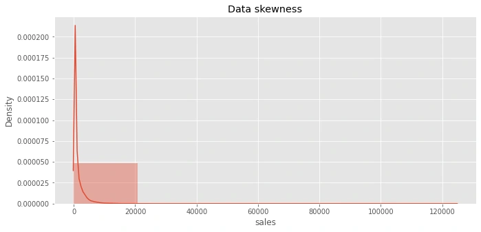
the sales are highly positively skewed, the given distribution is shifted to the left and with its tail on the right side.
Yearly average sales by: day, week, month
Daily:

Weekly:

Monthly:

Weekday average sales:
there is an increase in sales every year that indicates a trend variable
every day of the year the sales =0 as shown from "Daily Avg, which means that the market is closed.
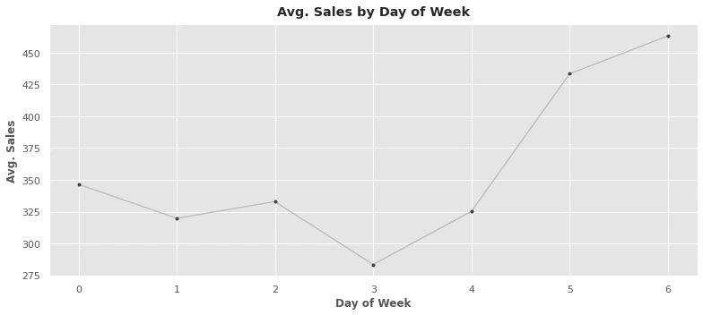
sales on the weekend the highest of the week and generally low on Thursdays.
Identifies the type of family product sold:
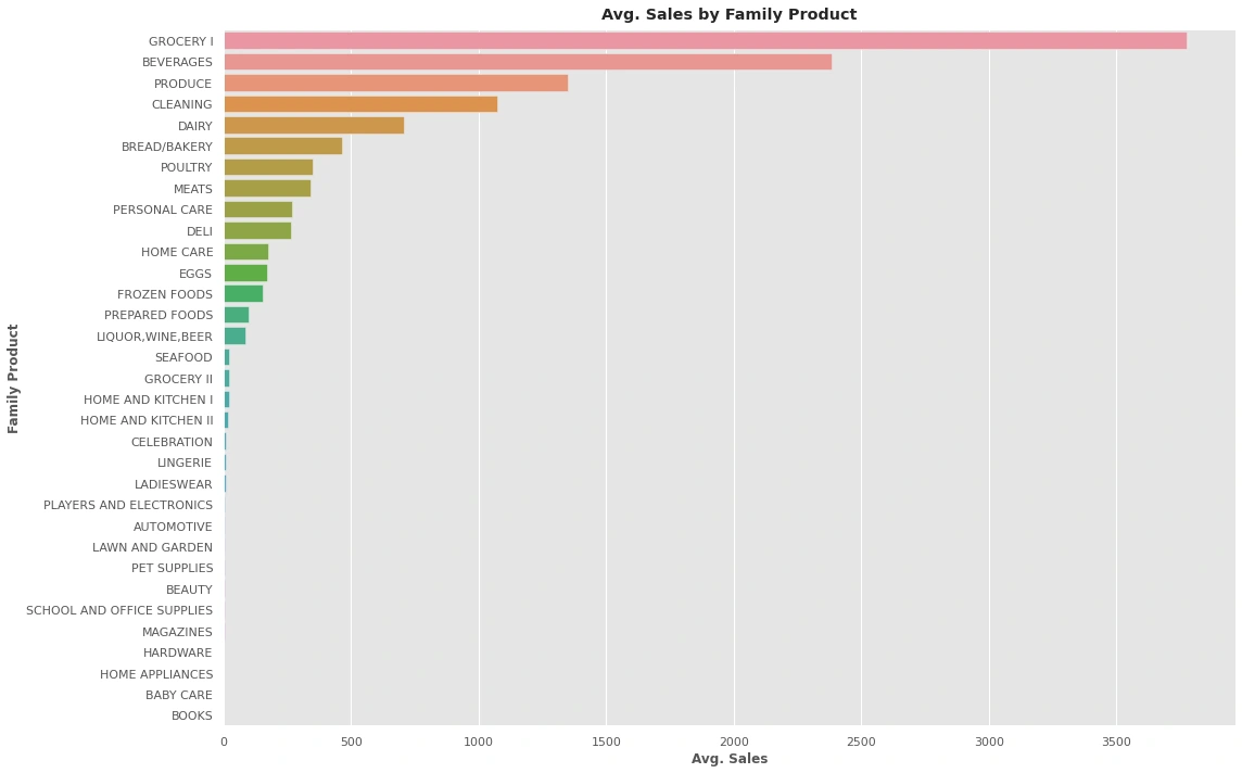
The best family products sell are: ['GROCERY I', 'BEVERAGES', 'PRODUCE', 'CLEANING', 'DAIRY']
The worst family products sell are: ['MAGAZINES', 'HARDWARE', 'HOME APPLIANCES', 'BABY CARE', 'BOOKS']
Identifies how the sales are going with each store:
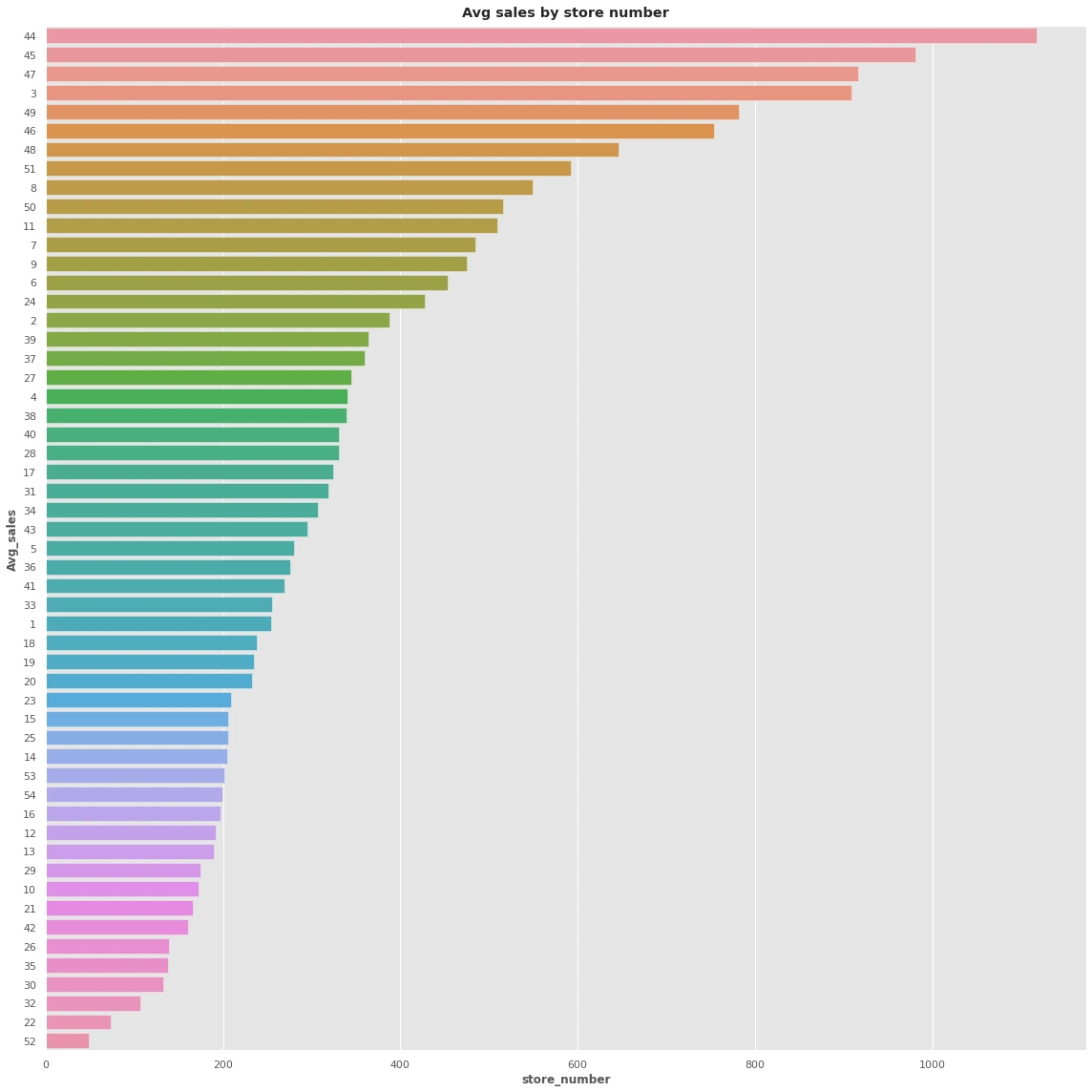
Best stores sales are : [44, 45, 47, 3, 49]
Worst stores sales are : [35, 30, 32, 22, 52]
Determine the trend
I choose a window of 365 days since this series has daily observations to smooth over any short-term changes within the year so that only the long-term changes remain
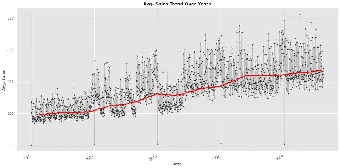
The sales is increasing over the years
Determine seasonality
Using the periodogram to determine the seasonality there are 10 different seasonalities Annual (1) Semiannual (2) Quarterly (4) Bimonthly (6) Monthly (12) Biweekly (26) Weekly (52) Semiweekly(104) Daily(365) Time of day
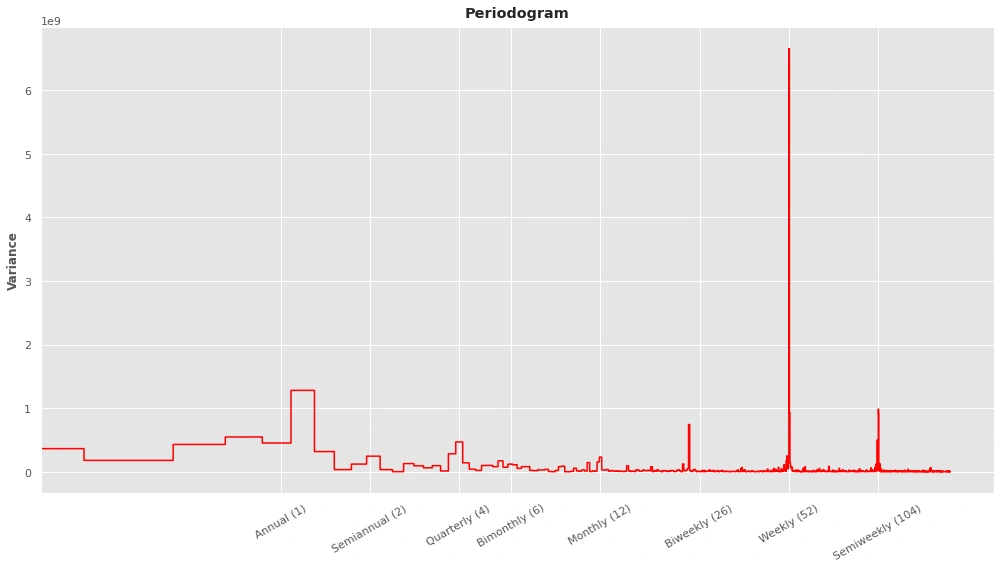
The periodogram suggests a strong weekly seasonality
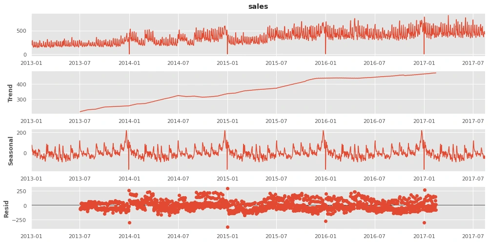
A lag plot of a time series shows its values plotted against its lags. Serial dependence in a time series will often become apparent by looking at a lag plot.
Using plot_pacf to see the correlation between 12 lags only:
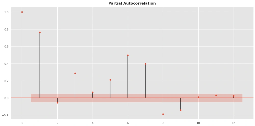
plot_pacf shows a strong correlation between lags (1 3 5 6 7 8 and 9) so we will be using these lags in training
Holidays
After removing the transferred data so it dont causes mislead the sales showed s strong correlation with sales:
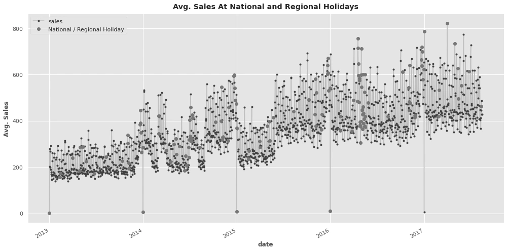
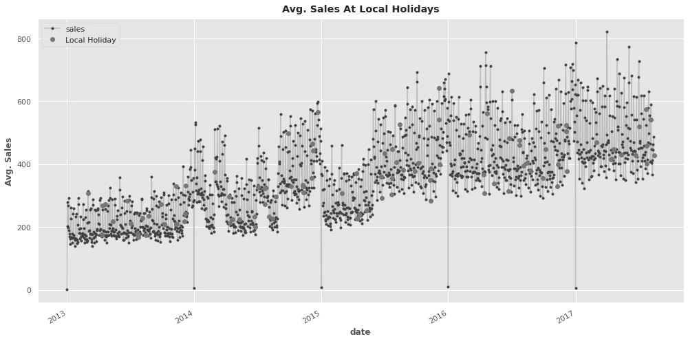
Comparing Avg_sales on holidays vs on workdays
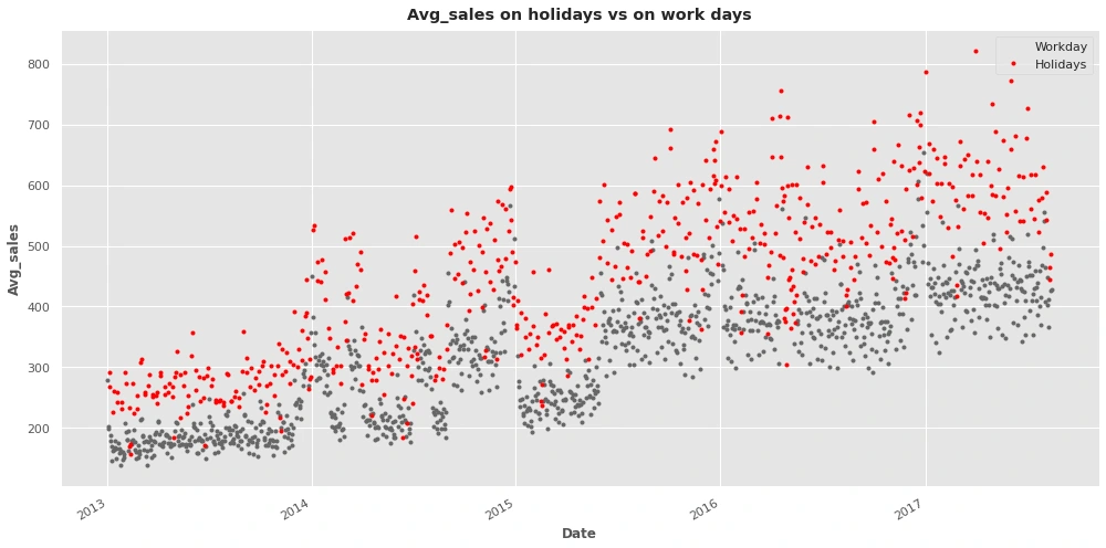
Sales are significantly higher in Holidays
Oil prices
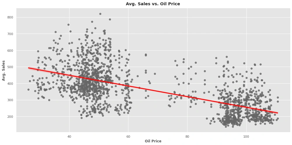
The oil price has a negative correlation with sales the lower the oil price is the more purchasing power for the customers.
Stores
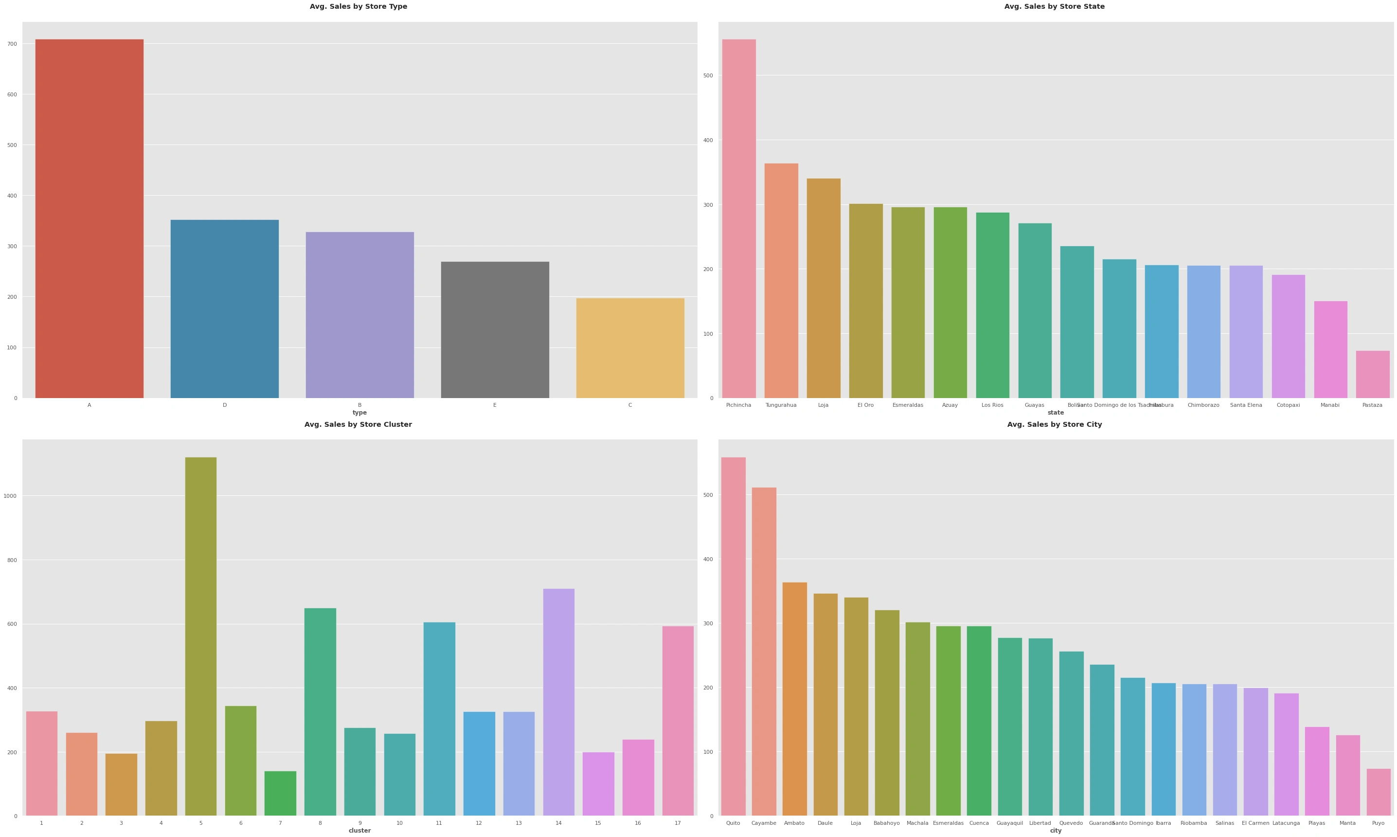
the plots show:
the best city sales are 'Quito' with over 500 and a percentage of 9.4% of total sales the lowest city sales is 'Puyo' with below 100 sales with only 1.2%
the order of best store type sales is (A, over(700),38% of sales),(B, over(300),19% of sales),(E,(300),17% of sales),(C, over(200),10.7% of sales)
the highest sale state is 'pichincha' with 13.2% of the sales and over 500 while the other states are close in sales with the highest percentage of 8.7 ('tungurahua') and the lowest is 'pasta' at 1.8%
the highest store cluster is 5 with over 1000 and a percentage of 16%
Modeling
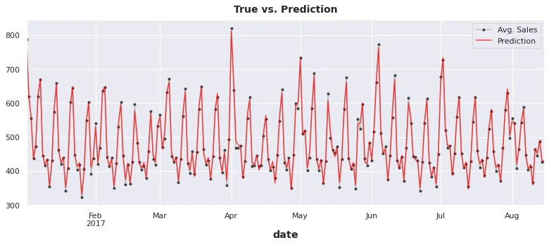
Linear regression excels at extrapolating trends, but can't learn interactions. CATBoost excels at learning interactions, but can't extrapolate trends. In the next codes, I'll create "hybrid" forecasters that combine complementary learning algorithms and let the strengths of one make up for the weakness of the other.
It's possible to use one algorithm for some of the components and another algorithm for the rest. This way we can always choose the best algorithm for each component. To do this, we use one algorithm to fit the original series and then the second algorithm to fit the residual series.
In detail, the process is this:
1-Train and predict with first model model_1.fit(X_train_1, y_train)
y_pred_1 = model_1.predict(X_train)
2-Train and predict with the second model on residuals
model_2.fit(X_train_2, y_train - y_pred_1)
y_pred_2 = model_2.predict(X_train_2)
And then Add to get overall predictions
y_pred = y_pred_1 + y_pred_2
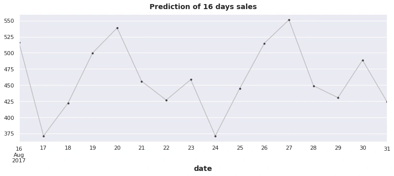
Forecasting the next 16 days' sales:
Like this project
Posted Jun 14, 2023
Contribute to Abdelrhman-Sadek/Store-chain-Analysis-and-Forecasting development by creating an account on GitHub.
Likes
0
Views
13


