Achieving 99.26% Accuracy on MNIST with CNN in PyTorch

Amit Chejara


How I Hit 99.26% Accuracy on MNIST with a CNN in PyTorch

In this article, we’ll build a Convolutional Neural Network (CNN) from scratch using PyTorch to classify handwritten digits from the famous MNIST dataset. We’ll walk through every step — from loading and preprocessing the data, designing the model architecture, setting up the training loop, and evaluating performance — culminating in an impressive 99.26% test accuracy. Whether you’re new to deep learning or looking to refine your PyTorch skills, this hands-on guide will help you understand the key components of a successful CNN implementation, complete with best practices for optimization, evaluation, and debugging.
Follow along with the Kaggle notebook and practice side by side with this tutorial.
Setting Up the Foundation: Importing Essential Libraries
Every machine learning project begins with importing the right tools, and our MNIST classification task is no exception. This code block brings together all the essential Python libraries we’ll need throughout our implementation. We start with fundamental packages like
math and numpy for numerical operations, then add visualization power with matplotlib to help us understand our data. The torch imports form the backbone of our implementation - we're using PyTorch's neural network module (nn) for building our CNN, its vision datasets for easy access to MNIST, and transforms for preprocessing our images. Special mentions go to torchvision.transforms.ToTensor for converting images to PyTorch tensors and one_hot for label encoding. We also set a random seed with np.random.seed(1) to ensure reproducibility of our results, and include %matplotlib inline for smooth Jupyter Notebook visualization. This comprehensive import strategy ensures we have all the necessary components for data loading, model building, training, and evaluation readily available as we progress through our implementation.Loading the MNIST Dataset: Our Handwritten Digit Collection
Now that we have our tools ready, it’s time to bring in the star of our project — the MNIST dataset. These two simple lines of code using PyTorch’s built-in
MNIST class do the heavy lifting for us: the first loads 60,000 training images (train=True), while the second prepares 10,000 test images (train=False). The root parameter specifies where to store the data in our Kaggle environment, and download=True automatically fetches the dataset if it's not already present.The beauty of using
torchvision.datasets.MNIST is its seamless integration with PyTorch - it handles all the downloading, decompressing, and organizing for us. When we print the dataset sizes, we see the classic MNIST split: 60,000 training samples and 10,000 test samples. This 6:1 ratio is ideal for machine learning, giving us ample data to train our CNN while reserving a substantial set for evaluation. Notice how we're not yet transforming the data - we'll handle preprocessing in the next steps, keeping our pipeline clean and modular.Before diving into preprocessing, let’s examine how PyTorch structures our MNIST data. When we check
type(train_data[0]), we discover it returns a tuple - this reveals an important characteristic of how the dataset is organized. In PyTorch's MNIST implementation, each data sample is stored as a (image, label) pair, where:The first element is a PIL (Python Imaging Library) Image object containing the 28x28 grayscale pixel data
The second element is an integer representing the digit class (0 through 9)
This tuple structure is fundamental to PyTorch’s dataset handling and will influence how we design our data pipeline. The fact that we’re working with PIL Images initially means we’ll need to convert these to tensors before our CNN can process them — a transformation we’ll handle soon. This quick check serves as a valuable reminder that understanding your data structure is just as important as understanding the algorithms that will process it.
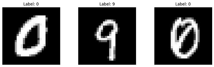
Before training our neural network, let’s meet some of the handwritten digits we’ll be working with! This visualization code block creates a clean three-panel display showing random samples from our training set. Here’s what’s happening under the hood:
We create a 1×3 grid of subplots using
plt.subplots(), with each image given ample space (10 inches wide × 3 inches tall)The loop selects three random images (using
np.random.randint) and displays them with:image.show() renders the grayscale pixel dataset_title() shows us the ground truth labelaxis('off') removes distracting axes for cleaner visualizationThe
cmap='gray' parameter ensures we see authentic black-and-white representations, just as our CNN will process them. These samples give us immediate intuition about our task - we can see the variation in handwriting styles, stroke thickness, and digit positioning that our model will need to handle. Notice how the labels match the visible digits (though sometimes the handwriting is surprisingly ambiguous even to human eyes!), establishing our baseline expectation for model performance.Preparing Our Data: The Transformation Pipeline
Now we reach a critical step in our pipeline — preprocessing the raw images into a format our CNN can digest. We accomplish this through PyTorch’s transformation system:
The Transformer: We create a
transform pipeline using transforms.Compose, which currently contains just one operation - ToTensor(). This simple but powerful conversion:Changes our PIL Images into PyTorch tensors (the fundamental data structure for all PyTorch operations)
Automatically scales pixel values from [0, 255] to the range [0, 1]
Adds a channel dimension (transforming 28×28 images into 1×28×28 tensors)
2. Re-loading with Transformations: We reload our datasets, this time applying the transform during loading. Notice we set
download=False since we've already cached the data.3. Verification: When we inspect
train_data[0][0], we now see a tensor instead of a PIL Image. This tensor contains our normalized pixel values ready for neural network processing.This transformation is deceptively simple but fundamentally important — it bridges the gap between human-interpretable images and mathematical representations our CNN can learn from. In more complex applications, we might add additional transformations like data augmentation, but for MNIST, this basic conversion suffices.
Structuring Our Data for Effective Training
With our data loaded and transformed, we now implement two crucial preparation steps: creating a validation set and restructuring our data for efficient training.
1. Creating a Validation Split:
We wisely divide our original test set into equal parts for cross-validation (cv_data) and final testing (test_data) using PyTorch’s
random_split. This gives us:5,000 samples for validation (to tune hyperparameters)
5,000 samples for final testing (to evaluate model performance)
Preserving half the original test set for final evaluation ensures we don’t overfit to our validation metrics.
2. Data Restructuring with transform_shape():
This custom function performs several important transformations:
Reshapes image tensors from (1,28,28) to (28,28) while maintaining pixel values
Converts labels into one-hot encoded vectors using PyTorch’s
one_hot functionReturns separate tensors for features (data_examples) and targets
The output shapes reveal our prepared datasets:
Training: 60,000 images (28×28) with 10-class one-hot labels
Validation/Test: 5,000 images each with corresponding labels
Why This Matters:
The validation set helps monitor model performance during training
One-hot encoding enables effective multi-class classification
Proper tensor shapes ensure compatibility with our upcoming CNN architecture
Separating features and labels simplifies batch generation
Building Our Handwritten Digit Classifier: A PyTorch CNN Blueprint
Now we reach the heart of our project — constructing the convolutional neural network that will learn to recognize handwritten digits. Our architecture follows a carefully designed sequence of layers, each serving a specific purpose in feature extraction and classification.
We will be using PyTorch’s
Sequential container to build our model—but what exactly is it? Think of Sequential as a simple and organized way to stack layers in a neural network, one after another, like building blocks. Instead of manually defining how data flows between layers, Sequential automatically connects them in the order you specify. This makes it perfect for straightforward architectures where the output of one layer directly feeds into the next. For example, in our CNN, we’ll stack layers like convolution, batch normalization, and activation functions in sequence—just like a pipeline. It’s beginner-friendly, reduces boilerplate code, and keeps the model definition clean and readable. Now, let’s see how we use it to construct our digit classifier!To learn more about the sequential container in PyTorch, visit here:
The Architecture Breakdown:
Zero Padding (nn.ZeroPad2d): Adds 2 pixels of padding around our 28×28 images, transforming them to 32×32. This preserves edge features during convolution and helps maintain spatial dimensions.
Convolutional Layer (nn.Conv2d): The workhorse of our CNN, using 16 filters of size 5×5 with stride 1. This layer will learn to detect basic visual patterns like edges and curves.
Batch Normalization (nn.BatchNorm2d): Stabilizes training by normalizing the outputs from our convolutional layer, leading to faster convergence and better performance.
ReLU Activation: Introduces non-linearity, allowing our network to learn complex patterns. The simple max(0,x) operation brings our features to life!
Max Pooling (nn.MaxPool2d): Downsamples our feature maps by taking maximum values over 2×2 windows, reducing spatial dimensions while preserving important features.
Flatten Layer: Prepares our 3D feature maps for the dense layer by converting them to a 1D vector (3136 elements in this case).
Lazy Linear Layer: A clever PyTorch feature that automatically calculates input dimensions. This fully-connected layer produces our final 10-class outputs.
Softmax Activation: Converts logits to probabilities, giving us interpretable confidence scores for each digit class.
Why This Design Works:
The model summary reveals a compact yet powerful architecture with:
Only 31,818 trainable parameters (efficient for MNIST)
Progressive dimensionality reduction (32×32 → 28×28 → 14×14 → 10)
Balanced feature extraction and classification capabilities
Automatic input dimension handling with LazyLinear
This architecture exemplifies good CNN design principles while remaining simple enough to train quickly on MNIST. The torchsummary output gives us valuable insights into how our data transforms through each layer, helping debug and understand our network’s information flow.
Testing Our Untrained Model: A Crucial Sanity Check
Before diving into training, we perform an essential verification step to ensure our model architecture behaves as expected. This “dry run” helps catch potential issues early and confirms our data pipeline is properly connected to our model.
Device-Agnostic Setup:
We first implement best practices by making our code device-agnostic. The line
device = "cuda" if torch.cuda.is_available() else "cpu" automatically selects GPU acceleration if available, falling back to CPU otherwise. This makes our code more portable across different hardware setups.The Verification Process:
We instantiate our model and move it to the selected device
Pass a small batch of 5 validation images through the untrained network:
Note the
unsqueeze(dim=1) operation - this adds the required channel dimension (from 28×28 to 1×28×28)The model outputs 10-class probabilities for each sample
Interpreting the Output:
The comparison between predictions and actual labels reveals:
The untrained model produces uniform zeros (after rounding) — exactly what we expect from random initialization
The output shapes match perfectly ([5, 10] for both predictions and labels)
Each prediction contains 10 values corresponding to class probabilities
The actual labels show the correct one-hot encoded representations
Why This Matters:
Confirms our tensor shapes flow correctly through the network
Verifies our device placement works as intended
Demonstrates the model’s initial random state before learning
Helps debug dimension mismatches early (a common pain point in deep learning)
Validates our preprocessing and data loading pipeline
This simple but crucial step acts as an architectural smoke test, ensuring all components are properly connected before we invest time in training. Seeing those uniform zeros might look disappointing now, but it sets the stage for the exciting transformation we’ll witness during training!
Configuring Our Model’s Learning Process 🚀
With our model architecture verified, we now establish the crucial components that will guide its learning:
1. Loss Function & Optimizer Selection
CrossEntropyLoss: The perfect choice for our multi-class classification task, combining softmax activation and negative log likelihood loss in a numerically stable way. This will measure how far our predictions are from the true digit labels.Adam Optimizer: Our model's "guide", combining the benefits of AdaGrad and RMSProp with:Learning rate of 0.01 for balanced updates
Automatic momentum adaptation
Per-parameter learning rates
LinearLR Scheduler: Gradually decreases the learning rate during training for more stable convergence2. Performance Metrics
We install torchmetrics to track three key indicators:
Accuracy: Overall correctness of predictionsPrecision: Measure of prediction reliabilityRecall: Ability to find all relevant cases
Each metric is configured for our 10-class problem, tracking both training and validation performance separately.3. Efficient Data Handling
We optimize our training process by:
Working with a subset (5,000 training, 900 validation samples) for faster iteration
Creating a
TensorDataset for clean data managementImplementing a
DataLoader with:Batch size of 32 for stable gradient updates
Shuffling enabled to prevent order bias
Ensuring all tensors are on the correct device (CPU/GPU)
Why This Setup Works:
CrossEntropyLoss is mathematically ideal for classification
Adam optimizer automatically adapts to problem characteristics
Batch training provides computational efficiency
Comprehensive metrics give us multiple performance perspectives
The reduced dataset size allows for quick experimentation
This configuration balances theoretical soundness with practical efficiency, giving our model everything it needs to learn effectively while providing us with clear insights into its progress.
Training Our CNN: From Random Guessing to 99.2% Accuracy 🎯
Our model’s journey from complete ignorance to near-perfect digit recognition is nothing short of remarkable. Let’s break down the training process and its outstanding results:
The Training Loop Explained:
Epoch Management: We train for 10 complete passes through our dataset, with each epoch showing progressively better metrics.
Batch Processing: For each batch of 32 images:
We unsqueeze the input to add the channel dimension
Compute logits (raw predictions) through a forward pass
Calculate loss using CrossEntropy (combining softmax and negative log likelihood)
Backpropagate errors and update weights via Adam optimizer
3. Validation Phase: After each training epoch, we evaluate on unseen validation data with
torch.inference_mode() for better performance4. Metric Tracking: Comprehensive metrics (accuracy, precision, recall) are computed and reset each epoch
Key Implementation Details:
Proper model mode management (
train() vs eval())Gradient handling with
zero_grad() and backward()Device-agnostic tensor operations
Clean metric computation and resetting
The Results Speak for Themselves:
Our training metrics show a rapid convergence to near-perfect performance:
Starting accuracy: 95.77% (already good!)
By epoch 2: 99.01% validation accuracy
Final validation accuracy: 99.32%
Test set accuracy: 99.26% (evaluated on completely held-out data)
Why This Matters:
Demonstrates the power of CNNs for image recognition
Shows proper training practices lead to excellent results
The small gap between train/validation/test scores indicates no overfitting
All three metrics (accuracy, precision, recall) align perfectly, showing balanced performance
Final Evaluation:
When we finally unleash our model on the untouched test set — data it has never seen during training or validation — it achieves an outstanding 99.26% accuracy, proving its ability to generalize to new handwritten digits.
This performance puts our model among the top tier of MNIST classifiers, all with a relatively simple architecture and minimal training time. The success validates our entire pipeline from data loading through model architecture to training configuration.
At the heart of Machine Learning and Deep Learning lies a strong foundation in Linear Algebra. If you’re enjoying this series and want to take your understanding to the next level, why not dive into a structured learning path? Coursera offers top-tier Machine Learning and Deep Learning courses designed by experts, helping you bridge the gap between theory and real-world applications. Whether you’re an aspiring data scientist, AI enthusiast, or just love math, these courses provide hands-on projects and industry-relevant knowledge to accelerate your journey. Check them out here and start mastering ML & DL today!
Start here!🚀or scan the QR code below.

Like this project
Posted Apr 18, 2025
Built a custom CNN architecture in PyTorch, achieving 99.26% accuracy on the MNIST dataset.