A/B Test Analyzer

Mo Rahman



🧪 A/B Test Analyzer
Rigorous experiment analysis from first principles — hypothesis tests, multiple-comparison correction, and power analysis implemented from the math, then verified by Monte Carlo simulation.
▶︎ Live demo — click Load demo data and press Run analysis; no CSV needed.
📄 Full technical report (PDF) — statistical foundations, pipeline design, and Monte Carlo validation write-up.
Why this exists
A product manager finishes an experiment, opens a spreadsheet with 15 metrics, and calls anything under p = 0.05 a win. Two things quietly go wrong:
Multiplicity. Testing 15 metrics at α = 0.05 gives a ~54% chance of at least one false positive. My simulations put the realized family-wise error rate at 57.6% for 20 metrics.
Underpowered nulls. "Not significant" gets read as "no effect," when often the experiment never had the sample size to see the effect at all.
This tool does the statistics correctly and says so in plain language. Every test, correction, and power calculation is implemented from the formulas — SciPy and statsmodels appear only in the test suite, as independent implementations to check against.
The demo dataset makes the point concretely:
support_tickets is a planted true null that lands at raw p = 0.042 — "significant" by the naive rule. Benjamini-Hochberg adjusts it to 0.062 and correctly leaves it alone.What it does
Two-sample tests Welch's t (default), Student's pooled t, Mann-Whitney U — auto-selected per metric from normality diagnostics, or overridden by the user Multiple comparisons Bonferroni (FWER) and Benjamini-Hochberg (FDR), both implemented from scratch Effect sizes Hedges' g with bootstrap CIs, rank-biserial r, common-language effect size P(T > C) Power Exact noncentral-t power, required sample size, and minimum detectable effect — not post-hoc power Diagnostics Shapiro-Wilk (subsampled at large n), skewness, Levene's test, with the test-selection reason surfaced per metric Output Interactive Streamlit UI plus a downloadable, self-contained HTML report
Screenshots
Verified, not just written
Unit tests check arithmetic.
simulations/validate_engine.py checks the statistical guarantees.Type I error calibration — 10,000 A/A experiments per setting:
Setting A/A rejection rate 95% CI Welch, normal data, n = 100/group 0.0530 0.0440 – 0.0637 Welch, lognormal data, n = 15/group 0.0285 0.0221 – 0.0367 Mann-Whitney U, lognormal, n = 15/group 0.0450 0.0368 – 0.0550
Welch sits on the nominal 5% under normality. On heavily skewed data at small n it becomes conservative, while the rank test stays calibrated — which is the empirical justification for the auto-selection rule, not a rule of thumb copied from a textbook.
FWER / FDR control — 20 metrics (15 true nulls, 5 real effects at d = 0.3, n = 200):
Correction FWER FDR Avg. power on real effects none 0.576 0.145 0.842 Bonferroni 0.056 0.019 0.480 Benjamini-Hochberg 0.210 0.054 0.645
Read this carefully: BH's FWER is 0.21, not ≤ α — BH never promised family-wise control. It pins the FDR at 0.054 ≈ α while recovering a third more power than Bonferroni. That trade-off is the entire reason both are offered.
Power curves — empirical rejection rates vs. the analytic noncentral-t function agree to within 0.04 across d ∈ {0.2, 0.5, 0.8} and n from 10 to 640.
Reproduce it yourself:
Additionally: every from-scratch estimator is cross-validated against an independent implementation — Welch/Student against
scipy.stats.ttest_ind to 1e-10, Bonferroni and BH against statsmodels.multipletests (including tied p-values), and the power trio against TTestIndPower plus Cohen's published benchmark (d = 0.5, α = 0.05, power = 0.8 ⟹ n = 64 per group, reproduced exactly). 360 tests, >90% coverage, CI on Python 3.10/3.11/3.12.Quickstart
Or with Docker:
Or use the engine directly, without the UI:
Input format — one row per randomization unit, one column identifying the group, one column per metric:
user_id group revenue_per_user session_minutes u000001 control 0.00 7.2 u000002 treatment 34.51 11.9
Methodology
Welch by default. Welch's t equals Student's t when variances are equal and stays valid when they aren't. Pre-testing variances with Levene and branching on the result distorts the error rate of the test that follows, so Levene is reported as context and never used to switch tests.
Test auto-selection. Mann-Whitney U is recommended when Shapiro-Wilk rejects normality and (|skew| > 1 or min group n < 30). Non-normality alone isn't disqualifying — the CLT protects the t-test on means as n grows. Shapiro-Wilk runs on a seeded 5,000-row subsample at large n, where it otherwise flags trivial deviations as significant.
Mann-Whitney U tests stochastic dominance — P(T > C) ≠ 0.5 — not "a difference in medians." That reading requires a location-shift assumption the data rarely satisfies. Reported alongside it: rank-biserial r and the common-language effect size ("a random treatment user beats a random control user 55% of the time"), both tie-aware.
FWER vs. FDR. Bonferroni bounds the probability of any false positive under arbitrary dependence — right when one false claim is expensive, e.g. a single guardrail metric gating a launch. BH bounds the expected share of false discoveries, assuming independence or positive dependence — right when screening many metrics. See the simulation table above for what each costs in power.
MDE, not post-hoc power. Observed power is a deterministic, monotone function of the p-value; computing it after the fact adds no information (Hoenig & Heisey, 2001). The report instead states the minimum detectable effect at the achieved n, and flags non-significant metrics whose MDE is large: "treat 'no effect found' as 'underpowered', not 'no effect'."
Degenerate samples. Zero pooled variance is split into two cases rather than collapsed: constant-and-equal groups give an effect of exactly 0, while constant-but-unequal groups (perfect separation) give signed infinity. Returning 0 for the latter would be a silent false negative on the most extreme separation possible. Bootstrap resamples that hit the degenerate case are excluded from the percentiles, with a warning when they exceed 1% of draws — common on coarse Likert or count data.
Full write-up:
docs/methodology.md, or the complete technical report (PDF).Architecture
The engine has no dependency on Streamlit, and the UI computes nothing. Any interface — CLI, notebook, scheduled job — consumes the same
ExperimentReport.Limitations
Stated plainly, because knowing the boundary matters more than the feature list:
Fixed-sample design assumed. Repeatedly analyzing accumulating data ("peeking") inflates the false positive rate well past α. These results are valid for a single pre-planned analysis. Sequential / always-valid inference is not implemented.
Independent randomization units assumed. No handling of clustered assignment, repeated measures per user, or marketplace interference between treatment and control.
No variance reduction. CUPED and other pre-experiment covariate adjustments would materially tighten intervals and aren't here.
Binary metrics are handled generically through the same machinery rather than with a two-proportion z-test or chi-square.
Ratio metrics (e.g. revenue per session, where the denominator is itself random) need the delta method for correct variance; not implemented.
Roadmap
Two-proportion z-test for conversion metrics · CUPED · Benjamini-Yekutieli for arbitrary dependence · permutation tests · sequential testing with alpha spending · delta-method CIs for ratio metrics
License
MIT
Like this project
Posted Aug 23, 2026
Statistical engine for experiment analysis: hypothesis tests, FDR correction, and power analysis — verified via Monte Carlo simulation, 360 benchmark tests.
Likes
0
Views
0