Survival Analysis | R

KUMAR RAHUL
Estimate probability of turnover of employees
#Set working directory
setwd("C:/Users/kumar/Desktop/ABA/Master")
#Read in data
#install.packages("readr")
library(readr)
survdat<-read.csv("Survival.csv")
names(survdat)
#create censoring variable
survdat$censored[survdat$Turnover==1]<-1
survdat$censored[survdat$Turnover==0|survdat$Turnover==2]<-0
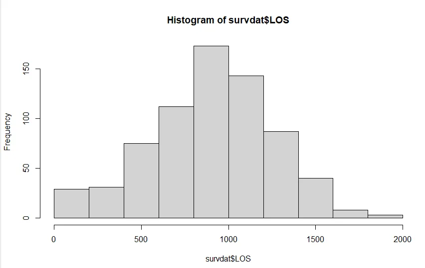
#Inspect Distribution of LOS Variable
hist(survdat$LOS)
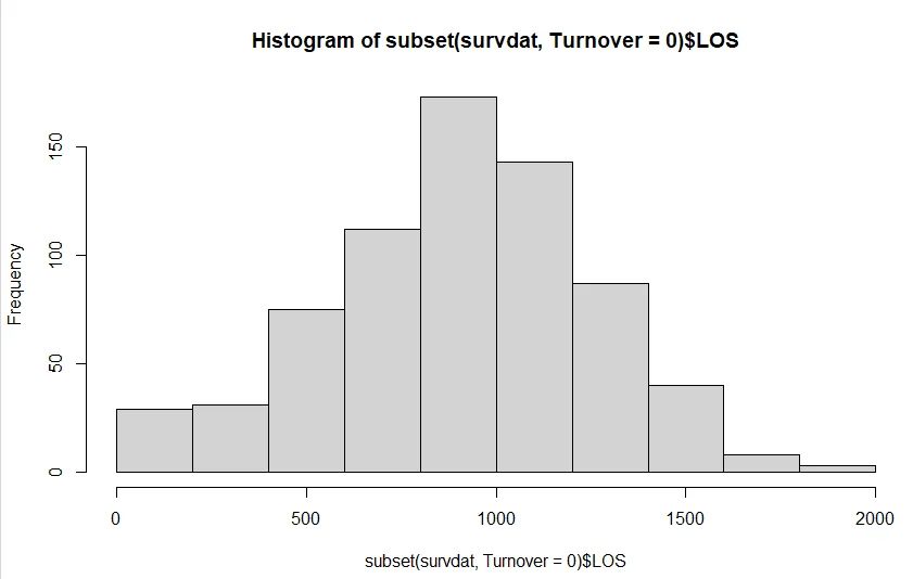
hist(subset(survdat,Turnover=0)$LOS)
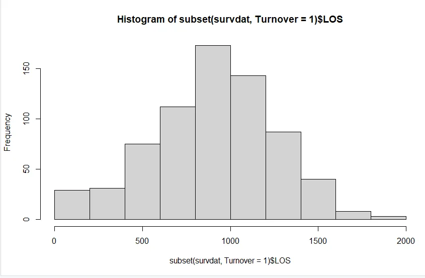
hist(subset(survdat,Turnover=1)$LOS)
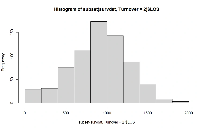
hist(subset(survdat,Turnover=2)$LOS)
#Kaplan-Meier Analysis(KM Analysis)- LifeTable
library(survival)
km_fit1<-survfit(Surv(LOS,censored)~1,
data=survdat,
type="kaplan-meier")
print(km_fit1)
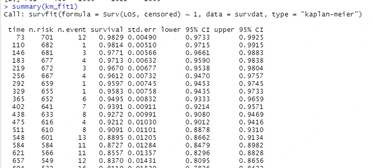
summary(km_fit1)
#summarize results by pre-specified time intervals
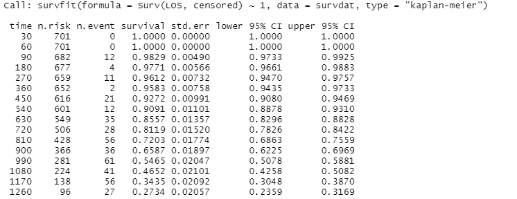
summary(km_fit1,times=c(30,60,90*(1:30)))
#install.packages(("survminer"))
library("survminer")
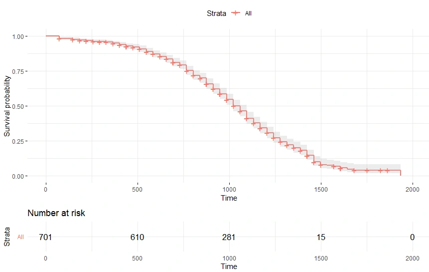
ggsurvplot(km_fit1,data=survdat,risk.table=TRUE,conf.int=TRUE,ggtheme=theme_minimal())
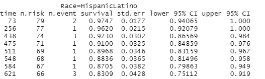
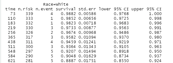
#Categorical KM Analysis:Race
km_fit2<-survfit(Surv(LOS,censored)~Race,
data=survdat,
type="kaplan-meier")
print(km_fit2)
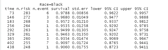
summary(km_fit2)
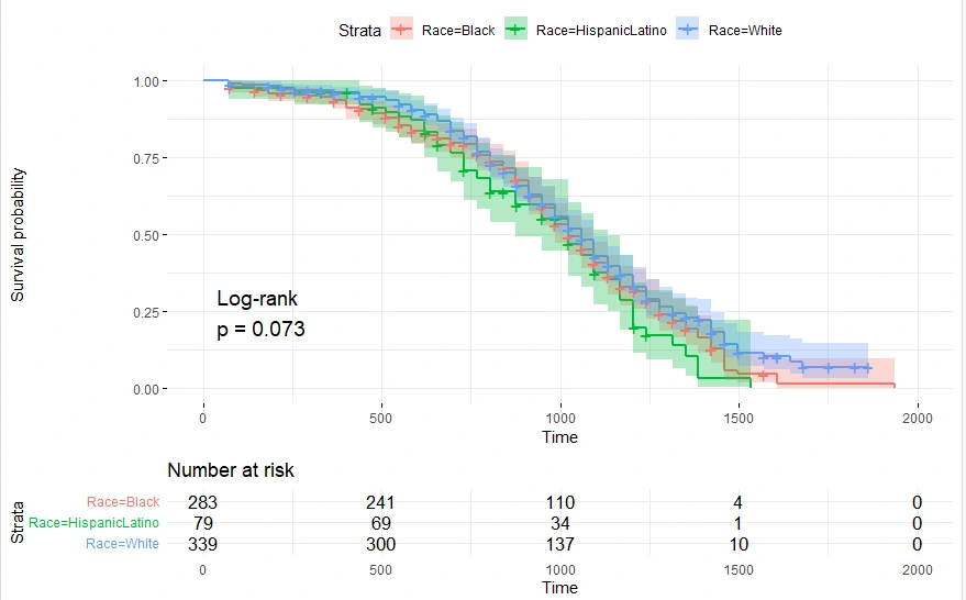
ggsurvplot(km_fit2,data=survdat,risk.table=TRUE,conf.int=TRUE,pval=TRUE,pval.method=TRUE,ggtheme=theme_minimal())ggsurvplot(km_fit2,data=survdat,risk.table=TRUE,conf.int=TRUE,pval=TRUE,pval.method=TRUE,ggtheme=theme_minimal())ggsurvplot(km_fit2,data=survdat,risk.table=TRUE,conf.int=TRUE,pval=TRUE,pval.method=TRUE,ggtheme=theme_minimal())ggsurvplot(km_fit2,data=survdat,risk.table=TRUE,conf.int=TRUE,pval=TRUE,pval.method=TRUE,ggtheme=theme_minimal())ggsurvplot(km_fit2,data=survdat,risk.table=TRUE,conf.int=TRUE,pval=TRUE,pval.method=TRUE,ggtheme=theme_minimal())ggsurvplot(km_fit2,data=survdat,risk.table=TRUE,conf.int=TRUE,pval=TRUE,pval.method=TRUE,ggtheme=theme_minimal())
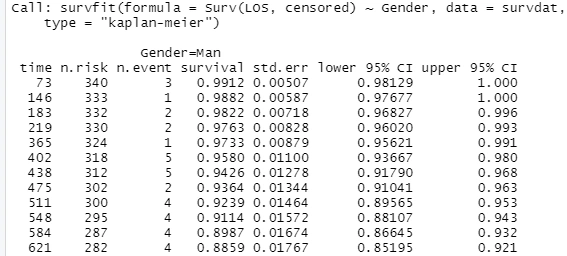
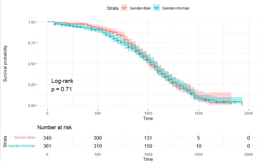
#Categorical KM Analysis: Gender
km_fit3<-survfit(Surv(LOS,censored)~Gender,
data=survdat,
type="kaplan-meier")
print(km_fit3)
summary(km_fit3)
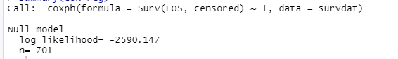
cox_reg<-coxph(Surv(LOS,censored)~1,data=survdat)#null-model
summary(cox_reg)
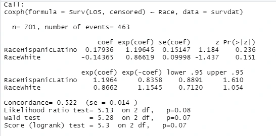
cox_reg1<-coxph(Surv(LOS,censored)~Race,data=dropna(survdat,LOS,censored,Race,Pay_hourly,Pay_sat))
summary(cox_reg1)
#Note1: Alphabetically, Black is the reference group.Survival Rate of survival of Hispanic Latino and white wrt to Black
#Note2: concordance is how well did the model predict how long people are going to survive before the event.
#Note3: logrrank test compares model with covariate with model with no covariate/null model
#Obsv1: Since the p-values>0.05, the variables are insignificant. Therefore, we do not discuss the hazard wrt to them.
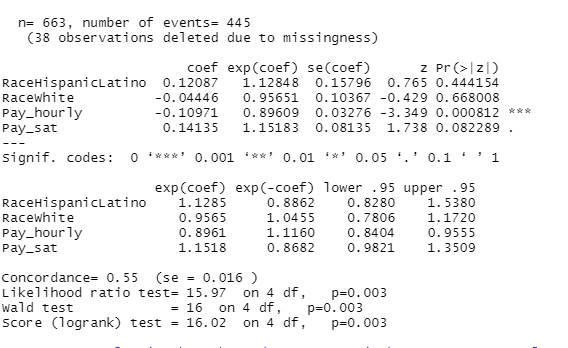
cox_reg2<-coxph(Surv(LOS,censored)~Race+Pay_hourly+Pay_sat,data=dropna(survdat,LOS,censored,Race,Pay_hourly,Pay_sat))
summary(cox_reg2)
#Note1: Sample size has changed to 663. It is because Pay_sat column has missing values.
#Obsv1: Hourly pay is significant. It is negative.Since it is significant,we look at the hazard ratio.
#1- hazard ratio=1-0.8961=0.1039. Interpretably,The risk of an individual voluntarily turning over/experiencing the focal
#event is going to decrease by 10.4% for every additional $ in hourly pay that the individual actually earns
#Application of the regression model
RaceHL=1#ishispaniclatino
RaceW=0
PH=16.00
PS=4.00
Log_overallrisk=.121*RaceHL-0.044*RaceW-0.109*PH+0.14135*PS
print(exp(Log_overallrisk))
#Risk of this individual turning over is 0.347.This individual is 65.27% less likely to quit when compared to individual
#with scores of 0 on each of the covariance in the model. But in reality Pay_Hourly and Pay_sat cannot be 0.
#Therefore, we mean-center the covariates
survdat$c_Pay_hourly<-scale(survdat$Pay_hourly,center=TRUE,scale=FALSE)
survdat$c_Pay_sat<-scale(survdat$Pay_sat,center=TRUE,scale=FALSE)
#Also,change the reference group from black to HispanicLatino
survdat$HL_Race<-factor(survdat$Race,levels=c("Hispaniclatino","Black","White"))
cox_reg3<-coxph(Surv(LOS,censored)~HL_Race+c_Pay_hourly+c_Pay_sat,data=dropna(survdat,LOS,censored,Race,Pay_hourly,Pay_sat))
summary(cox_reg3)
RaceB=0
RaceW=0
PH=16.00-mean(survdat$Pay_hourly,na.rm=TRUE )#na.rm will drop the missing data
PS=4.00-mean(survdat$Pay_sat,na.rm=TRUE)
Log_overallrisk=.121*RaceB-0.044*RaceW-0.109*PH+0.14135*PS
print(exp(Log_overallrisk))
##Risk of this individual turning over is 0.851.This individual is 14.8% less likely to quit when compared to individual
#with scores of 0 on dummy variables and mean Pay_hourly and Pay_Sat
library(tidyr)
anova(cox_reg,cox_reg1)#number of observations should be same
Like this project
Posted Feb 11, 2022
Estimate probability of turnover of employees
Likes
0
Views
3
Tags